There is a repo associated with this blog post here
There is a blog post that explains the Ad Analytics code example used below here
Introduction
We recently released a mixed workload example for Ad Analytics (description and source code on github) to illustrate the simplicity of development using SQL or the Spark Dataframe API in SnappyData. By mixed workload we mean a system that that is continuously ingesting a high velocity stream of ad impressions while concurrently serving ad-hoc interactive queries. In addition to demonstrating SnappyData’s simplicity, we wanted to also benchmark it against alternatives. Here we try to understand SnappyData’s performance compared to alternate “lambda” stacks - Cassandra + Spark and MemSQL + Spark for both stream ingestion rate and interactive analytic query performance.
Our summarized findings:
- Snappydata can ingest data twice as fast as Cassandra and 1.5 times faster than MemSQL.
- While ingesting data, SnappyData can concurrently execute analytics class queries 45 times faster than Cassandra and 3 times faster than MemSQL.
Note that these numbers represent queries over exact datasets; they do not include SnappyData’s Approximate Query Processing techniques. When these techniques are used (and the data volumes have grown), query latency becomes multiple orders of magnitude faster. The source code used for these tests is available on Github. Below, we will describe the benchmark:
Machine Configuration
Five ‘c4.2xlarge’ Compute optimized EC2 instances with
- 8 Cores
- 15GB RAM
- Dedicated EBS bandwidth of 1000 Mbps
Product versions used:
MemSQL
- MemSQL Ops-4.1.11 Community Edition
- Spark-MemSQL Connector 2.10_1.3.2
- Spark 1.5.2
Cassandra
- Cassandra 3.5
- Spark-Cassandra Connector 2.10_1.6.0-M2
- Spark 1.6.0
- SnappyData
- SnappyData 0.3-PREVIEW; with Spark 1.6.1 is bundled
- Apache Kafka 2.10_0.8.2.2.
Architecture
One machine was used for the Spark Master while the other four were used as Workers. A single Kafka producer process was executed producing ad impressions (asynchronously) over 16 threads. Four Kafka brokers were collocated on the Spark Worker nodes. We used 32 Kafka partitions to maximize concurrent processing. The kafka producer uses Avro Java objects to represent AdImpressions. Each AdImpression, when serialized, has a payload size of 63 bytes. To allow for concurrent analytical queries we configured spark so enough cores were available for query processing.
Finally, each tested system used the highest version of Spark it supported: 1.6.1 for SnappyData, 1.6.0 for Cassandra and 1.5.2 for MemSQL.
For each store that supported columnar storage, we used a column store to support fast scans and aggregations. Data is ingested using the Kafka direct receiver available with Spark Streaming and ingested in parallel on each partition.
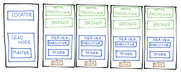
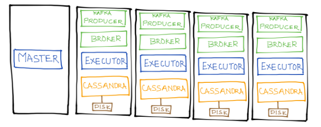
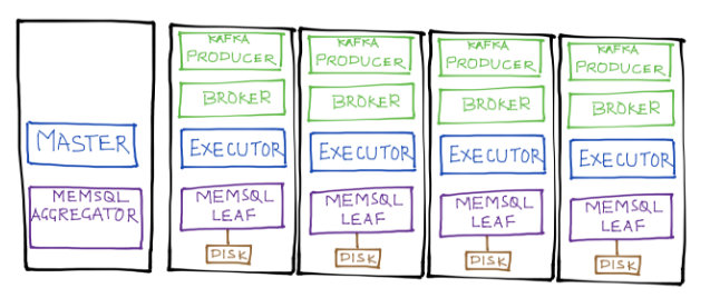
The figures below depict the benchmark architecture for all 3 product configurations. The only difference with SnappyData is that its store is fully collocated with the spark executors as depicted in the figure here. SnappyData completely avoids the need to shuffle data as its column store defaults to the partitioning used by the upstream RDD (Spark DStream in this case) resulting in better speed of ingestion and query performance.
SnappyData
We ran the locator and the lead node (which runs the Spark Driver and is the cluster master) on one server and used the remaining four to parallel ingest from kafka and store into the column table (both in-memory and on disk).
Spark-Cassandra
Similar to SnappyData we run the spark master/Driver on one node and so the ingestion process on the remaining 4 AWS nodes.
Spark-MemSQL
Matching what we did for SnappyData we start the spark master/Driver along with the MemSQL aggregator on one node and the remaining nodes parallely ingest and store into a local column table in MemSQL.
Cassandra Tuning
To tune writes, the cassandra connector batches incoming writes and exposes several tuning parameters. The ones we adjusted are listed above. Given the number of cores in use, adjusting the concurrent writer count gave us the maximum throughput. By default, the connector retains up to 1000 batches per single Spark task in memory before writing to Cassandra. This configuration is inappropriate in a production scenario unless checkpointing is enabled in Spark Streaming. While we didn’t tune any memory setting in the Cassandra servers we ensured that enough memory was available on each node to ensure all the data will be cached in the OS page cache.
MemSQL Tuning
We used defaults for the MemSQL configuration.
SnappyData Tuning
We used defaults for SnappyData configuration.
Ingestion Performance
To ingest data we used the Spark streaming Kafka direct receiver. This is the most optimal way to fetch from kafka – batches from the topic are directly processed by the stream without any additional buffering in the Spark layer.
For all three products, each incoming Avro message is first decoded and then turned into a Spark Row object before it is stored into their respective Column table (in-memory + disk persistent). Below is the code snippet used to store streaming data into a column table in SnappyData.
In the Cassandra case, we ingest into a table with no replication (i.e. replication factor 1) so it is equivalent to Snappydata.
In the MemSQL case, we created the equivalent column table:
And stored the incoming streaming data into the coulmn table:
The chart below shows the ingestion per second throughput after some warm up period.
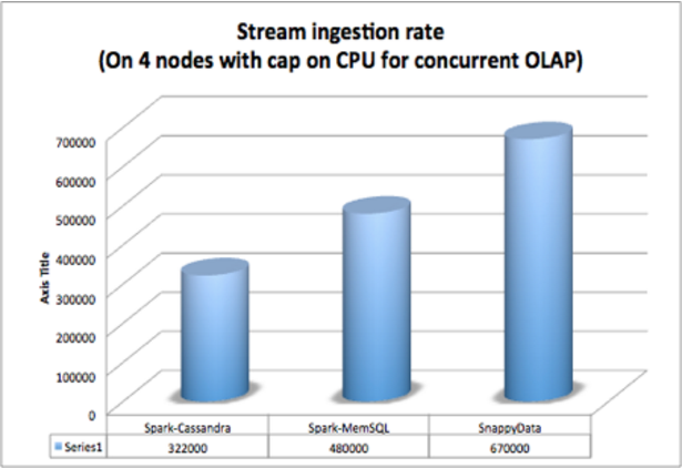
In short, on 4 nodes with 8 cores and a capped CPU (to leave space for concurrent OLAP queries), SnappyData outperformed Spark-Cassandra by roughly 2x with 670,000 events per second versus 322,000 and outperformed MemSQL by roughly 1.5x with 670,000 vs 480,000.
Concurrent Query workload
We concurrently execute simple aggregation queries using the Spark SQL Driver program when the ingested data reaches 30, 60 and 90 million records. We logged the query execution time to a file. For example, you can see the driver program for Cassandra here. We used following three aggregation queries to measure OLAP performance.
Q1 : Show top 20 Geos with the highest ad impressions
select count(*) AS adCount, geo from adImpressions group by geo order by adCount desc limit 20;
Q2: Geos with the highest total bid
select sum (bid) as max_bid, geo from adImpressions group by geo order by max_bid desc limit 20;
Q3: Top 20 publishers with the highest bid total
select sum (bid) as max_bid, publisher from adImpressions group by publisher order by max_bid desc limit 20;
The following chart shows the latency numbers for each query by product and row count.
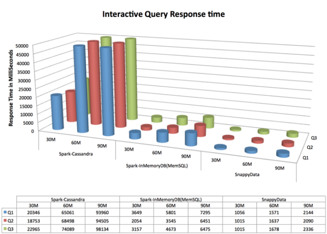
As you can see SnappyData outperforms Spark-Cassandra by roughly 45 times when executing queries while also ingesting data and outperforms MemSQL by roughly 3 times on the same setup.
Analysis
The Cassandra connector suffers from two problems:
- The full data has to be serialized and copied to the spark cluster including going through format conversions for each query and
- The data has to be shuffled across multiple partitions.
These issues add latency to both ingestion and query performance.
The MemSQL connector, on the other hand, attempts to push as much of the query as possible to MemSQL which provides significant savings in having to move large quantities of data into Spark for each query. Go through MemSQLPushdownStrategy and MemSQLPhysicalRDD for details. The other optimization in MemSQL is that it always attempts to collocate its partition to the parent, so, kafka partitions, queuing, and ingestion all occur without ever having to shuffle any records.
SnappyData embeds its column store alongside the Spark executors providing reference level access to rows. Similar to MemSQL, it also ensures that each partition in the store layer, by default, uses the parent’s partitioning method. i.e. there is no need to shuffle during storing. When queried, the data is column compressed and formatted in the same format as Spark (when cached or persisted). These features provide a significant performance boost in ingestion and query latency.
Interactive Query response with AQP
We also benchmarked SnappyData’s Approximate Query Processing techniques and compared this to “exact” queries against our in-memory column tables. While these sampling techniques require large data volumes for higher accuracy, we compensated by creating a relatively large stratified sample of 3% to work with smaller data sets in this example. We created a sample on the base column Table. When queries are executed we append an error clause so the sample is automatically consulted (‘select .. from aggrAdImpressions group by … with error 0.2’). Let’s compare our 3 queries over the exact table and sample table (In SnappyData) at 350m, 400m and 450m records with concurrent streaming.
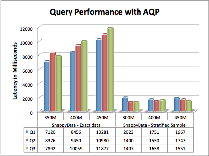
As expected, the sample table execution is much faster than its counterpart exact table. While the performance is high, usually with large data sets the sample fraction can be much smaller with a resulting performance difference that is 2 or even 3 orders of magnitude better than running against the base table. It is also interesting to note that, with increasing data volume, the query execution time on the sample stays fairly constant. While the sample size grows in proportion to the base table size, most of the query execution cost comes from other sources like error computation and query planning through the spark driver. Other performance related blogs:
SnappyData is available for download.
Learn more and chat about SnappyData on any of our community channels:
Stackoverflow
Slack
Mailing List
Gitter
Reddit
JIRA
Other important links:
SnappyData source
SnappyData docs
SnappyData twitter
SnappyData technical paper

