Geospatial Anomaly Detection (Terra-Locus Anomalia Machina) Part 2: Geohashes (2D)

Massively Scalable Geospatial Anomaly Detection with Apache Kafka and CassandraIn this blog, we continue exploring how to build a scalable Geospatial Anomaly Detector. In the previous blog, we introduced the problem and tried an initial Cassandra data model with locations based on latitude and longitude. We now try another approach, Geohashes, to start with, of the 2D kind, and have some close encounters of another kind (Space vs. Time). Note that Geohashes are easily confused with Geohashing, which is an outdoor adventure sport based on trying to reach a random Geohash, and Geocaching, which is a worldwide treasure hunt to attempt to find geocaches hidden at different locations. So, on with the adventure of the Geohashes kind!In the previous blog (Geospatial Anomaly Detection: Part 1) we discovered that efficient proximity querying over <latitude, longitude> location coordinates using inequalities is challenging in Cassandra.Is there an alternative?  Perhaps the experiments in the previous blog, using a country string as the partition key, give us a valuable clue? The Earth can be divided up in a lot of different (but somewhat arbitrary) ways such as by countries, continents, or even tectonic plates!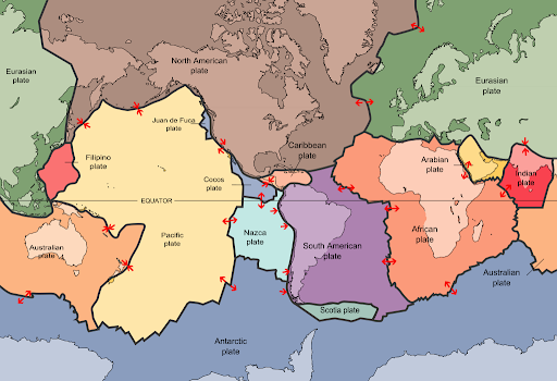The major tectonic plates  (Source: Wikipedia)What if there was a more “scientific” way of dividing the world up into different named areas, ideally hierarchical, with decreasing sizes, with a unique name for each? Perhaps more like how an address works. For example, using a combination of plate, continent, and country, what famous building is located here?North American Plate ->Continent of North America ->U.S.A. ->District of Columbia ->Washington ->Northwest ->Pennsylvania Avenue ->1600“The” White House! Actually, tectonic plates are hierarchical, as there are major, minor and microplates (but only sometimes and at geological timescales).  It turns out that there are many options for systematically dividing the planet up into nested areas. One popular method is a Geohash. Geohashes use “Z-order curves” to reduce multiple dimensions to a single dimension with fixed ordering (which turns out to be useful for database indexing). A geohash is a variable length string of alphanumeric characters in base-32 (using the digits 0-9 and lower case letters except a, i, l and o), e.g. “gcpuuz2x” (try pronouncing that!) is the geohash for Buckingham Palace, London. A geohash identifies a rectangular cell on the Earth: at each level, each extra character identifies one of 32 sub-cells as shown in the following diagram.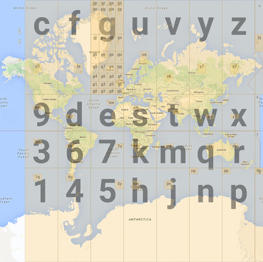(Source: moveable-type.co.uk)Shorter geohashes have larger areas, while longer geohashes have smaller areas. A single character geohash represents a huge 5,000 km by 5,000 km area, while an 8 character geohash is a much smaller area, 40m by 20m. Greater London is “gcpu”, while “gc” includes Ireland and most of the UK. To use geohashes you encode <latitude, longitude> locations to a geohash (which is not a point, but an area), and decode a geohash to an approximate <latitude, longitude> (the accuracy depends on the geohash length).  Some geohashes are even actual English words. You can look up geohashes online (which is an easier type of adventure than geohashing or geocaching): “here” is in Antarctica, “there” is in the Middle East, and “everywhere” is (a very small spot) in Morocco! And here’s an online zoomable geohash map which makes it easy to see the impact of adding more characters to the geohash.Geohashes are a simpler version of bounding boxes that we tried in the previous blog, as locations with the same geohash will be near each other, as they are in the same rectangular area. 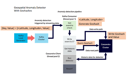However, there are some limitations to watch out for including edge cases and non-linearity near the poles.To use geohashes with our Anomalia Machina application, we needed a Java implementation, so we picked this one (which was coincidentally developed by someone geospatially nearby to the Instaclustr office in Canberra).  We modified the original Anomalia Machina code as follows. The Kafka key is a <latitude, longitude> pair. Once an event reaches the Kafka consumer at the start of the anomaly detection pipeline we encode it as geohash and write it to Cassandra. The query to find nearby events now uses the geohash. The modified anomaly detection pipeline looks like this:But how exactly are we going to use the geohash in Cassandra? There are a number of options.2.1 Geohash Option 1—Multiple Indexed Geohash ColumnsThe simplest approach that I could think of to use geohashes with Cassandra, was to have multiple secondary indexed columns, one column for each geohash length, from 1 character to 8 characters long (which gives a precision of +/- 19m which we assume is adequate for this example).The schema is as follows, with the 1 character geohash as the partition key, time as the clustering key, and the longer (but smaller area) geohashes as secondary indexes:In practice the multiple indexes are used by searching from smallest to largest areas. To find the (approximately) nearest 50 events to a specific location (e.g. 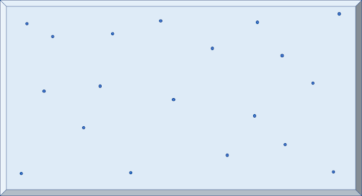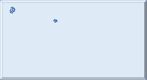“everywhere”, shortened to an 8 character geohash, “everywhe”), we start querying with smallest area first, the 8 character geohash, and increase the area by querying over shorter geohashes, until 50 events are found, then stop:Spatial Distribution and Spatial DensityWhat are the tradeoffs with this approach? The extra data storage overhead of having multiple geohash columns, the overhead of multiple secondary indexes, the overhead of multiple reads, due to (potentially) searching multiple areas (up to 8) to find 50 events, and the approximate nature of the spatial search due to the use of geohashes.  How likely we are to find 50 nearby events on the first search depends on spatial distribution (how spread out in space events are, broad vs. 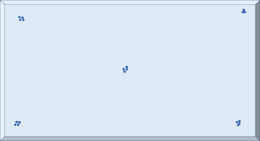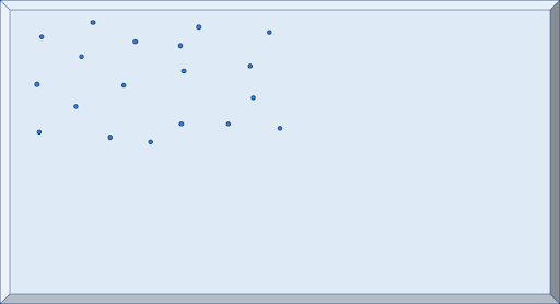narrow) and spatial density (how many events there are in a given area, which depends on how sparse or clumped together they are).For example, broad distribution and sparse density:Broad distribution and clumped:Narrow distribution and sparse:Narrow distribution and clumped:There’s a potentially nice benefit of using geohashes for location in our anomaly detection application.  Because they are areas rather than highly specific locations, once an anomaly has been detected it’s automatically associated with an area which can be included with the anomaly event reporting. This may be more useful than just a highly specific location in some cases (e.g. for setting up buffer and exclusion zones, triggering more sophisticated but expensive anomaly detection algorithms on all the data in the wider area, etc.). This is the flip side of the better-known fact that geohashes are good for privacy protection by virtue of anonymizing the exact location of an individual. Depending on the hash length the actual location of an event can be made as vague as required to hide the location (and therefore the identify) of the event producer.  Note that in theory, we don’t have to include the partition key in the query if we are using secondary indexes, i.e. this will work:The downside of this query is that every node is involved. The upside, that we can choose a partition key with sufficient cardinality to avoid having a few large partitions, which is not a good idea in Cassandra (see note below).2.2 Geohash Option 2—Denormalized Multiple TablesThere are a couple of different possible implementations of this basic idea. One is to denormalize the data and use multiple Cassandra tables, one for each geohash length. Denormalization by duplicating data across multiple tables to optimize for queries, is common in Cassandra—“In Cassandra, denormalization is, well, perfectly normal” – so we’ll definitely try this approach.We create 8 tables, one for each geohash length:For each new event, we compute geohashes from 1 to 8 characters long, and write the geohash and the value to each corresponding table.  This is fine as Cassandra is optimized for writes. The queries are now directed to each table from smallest to largest area geohashes until 50 events are found:2.3 Geohash Option 3—Multiple Clustering ColumnsDid you know that Cassandra supports multiple Clustering columns? I had forgotten. So, another idea is to use clustering columns for the geohashes, i.e. instead of having multiple indexes, one for each length geohash column, we could have multiple clustering columns:12345678910111213CREATE TABLE geohash1to8_clustering(geohash1 text,time timestamp,geohash2 text,gephash3 text,geohash4 text,geohash5 text,geohash6 text,geohash7 text,geohash8 text,value double,PRIMARY KEY(geohash1,geohash2,geohash3,geohash4,geohash5,geohash6,geohash7,geohash8,time))WITH CLUSTERING ORDER BY(geohash2 DESC,geohash3 DESC,geohash4 DESC,geohash5 DESC,geohash6 DESC,geohash7 DESC,geohash8 DESC,time DESC);Clustering columns work well for modeling and efficiently querying hierarchically organized data, so geohashes are a good fit, i.e. a single clustering column is often used to retrieve data in a particular order (e.g. for time series data) but multiple clustering columns are good for nested relationships, as Cassandra stores and locates clustering column data in nested sort order. The data is stored hierarchically, which the query must traverse (either partially or completely). To avoid “full scans” of the partition (and to make queries more efficient), a select query must include the higher level columns (in the sort order) restricted by the equals operator. Ranges are only allowed on the last column in the query. A query does not need to include all the clustering columns, as it can omit lower level clustering columns.Time Series data is often aggregated into increasingly longer bucket intervals (e.g. seconds, minutes, hours, days, weeks, months, years), and accessed via multiple clustering columns in a similar way.  However, maybe only time and space (and other as yet undiscovered dimensions) are good examples of the use of multiple clustering columns? Are there other good examples? Maybe organizational hierarchies (e.g. military ranks are very hierarchical after all), biological systems, linguistics and cultural/social systems, and even engineered and built systems. Unfortunately, there doesn’t seem to be much written about modeling hierarchical data in Cassandra using clustering columns, but it does look as if you are potentially only limited by your imagination.The query is then a bit trickier as you have to ensure that to query for a particular length geohash, all the previous columns have an equality comparison. For example, to query a length 3 geohash, all the preceding columns (geohash1, geohash2) must be included first:2.4 Geohash Option 4—Single Geohash Clustering ColumnAnother approach is to have a single full-length geohash as a clustering column. This blog (Z Earth, it is round?! In which visualization helps explain how good indexing goes weird) explains why this is a good idea:“The advantage of [a space filling curve with] ordering cells is that columnar data stores [such as Cassandra] provide range queries that are easily built from the linear ordering that the curves impose on grid cells.”Got that? It’s easier to understand an example:Note that we still need a partition key, and we will use the shortest geohash with 1 character for this. There are two clustering keys, geohash8 and time. This enables us to use an inequality range query with decreasing length geohashes to replicate the above search from smallest to largest areas as follows:(Source: Shutterstock)Just like some office partitions, there can be issues with Cassandra partition sizes. In the above geohash approaches we used sub-continental (or even continental scale as “6” is almost the whole of South America!) scale partition keys. Is there any issue with having large partitions like this?Recently I went along to our regular Canberra Big Data Meetup and was reminded of some important Cassandra schema design rules in Jordan’s talk (“Storing and Using Metrics for 3000 nodes—How Instaclustr use a Time Series Cassandra Data Model to store 1 million metrics a minute”)Even though some of the above approaches may work (but possibly only briefly as it turns out), another important consideration in Cassandra is how long they will work for, and if there are any issues with long term cluster maintenance and node recovery.  The relevant rule is related to the partition key. In the examples above we used the shortest geohash with a length of 1 character, and therefore a cardinality of 32, as the partition key. This means that we have a maximum of 32 partitions, some of which may be very large (depending on the spatial distribution of the data). In Cassandra, you shouldn’t have unbounded partitions (partitions that keep on growing fast forever), partitions that are too large (> 100MB), or uneven partitions (partitions that have a lot more rows than others). Bounded, small, even partitions are Good. Unbounded, large, uneven partitions are Bad. It appears that we have broken all three rules.However, there are some possible design refinements that come to the rescue to stop the partitions closing in on you, including (1) a composite partition key to reduce partition sizes, (2) a longer geohash as the partition key to increase the cardinality, (3) TTLs to reduce the partition sizes, and (4) sharding to reduce the partition sizes. We’ll have a brief look at each.3.1 Composite PartitionsA common approach in Cassandra to limit partition size is to use a composite partition key, with a bucket as the 2nd column. For example:The bucket represents a number of fixed duration time range (e.g. from minutes to potentially days), chosen based on the write rate to the table, to keep the partitions under the recommended 100MB. To query you now have to use both the geohash1 and the time bucket, and multiple queries are used to go back further in time. Assuming we have a “day” length bucket:Space vs. TimeBut this raises the important (and ignored so far) question of Space vs. Time. Which is more important for Geospatial Anomaly Detection? Space? Or Time?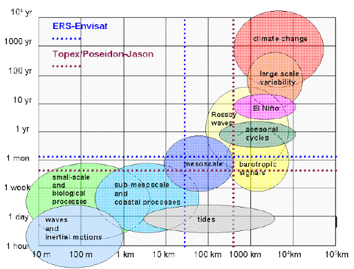Space-time scales of major processes occurring in the ocean (spatial and temporal sampling on a wide range of scales)  (Source: researchgate.net)The answer is that it really depends on the specific use case, what’s being observed, how and why. In the natural world some phenomena are Big but Short (e.g. tides), others are Small but Longer (e.g. biological), while others are Planetary in scale and very long (e.g. climate change).So far we have assumed that space is more important, and that the queries will find the 50 nearest events no matter how far back in time they may be.  This is great for detecting anomalies in long term trends (and potentially over larger areas), but not so good for more real-time, rapidly changing, and localised problems.  If we relax the assumption that space is more important than time, we can then add a time bucket and solve the partition size problem. For example, assuming the maximum sustainable throughput we achieved for the benchmark in Anomalia Machina Blog 10 of 200,000 events per second, 24 bytes per row, uniform spatial distribution, and an upper threshold of 100MB per partition, then the time bucket for the shortest geohash (geohash1) can be at most 10 minutes, geohash2 can be longer at just over 5 hours, and geohash3 is 7 days.What impact does this have on the queries? The question then is how far back in time do we go before we decide to give up on the current search area and increase the area? Back to the big bang? To the dinosaurs? Yesterday? Last minute?  The logical possibilities are as follows.We could just go back to some maximum constant threshold time for each area before increasing the search area. 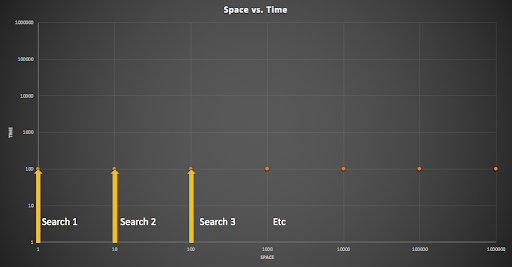For example, this diagram shows searches going from left to right, starting from the smallest area (1), increasing the area for each search, but with a constant maximum time threshold of 100 for each:Constant time search with increasing space searchAlternatively, we could alternate between increasing time and space.  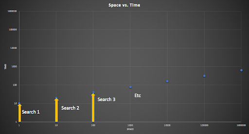For example, this diagram shows searches going from left to right, again starting from the smallest area and increasing, but with an increasing time threshold for each:Increasing time search with increasing space searchHowever, a more sensible approach (based on the observation that the larger the geohash area the more events there will be), is to change the time threshold based on the space being searched (i.e. time scale inversely depends on space scale). Very small areas have longer times (as there may not be very many events given in a minuscule location), but bigger areas have shorter times (as there will be massively more events at larger scales). 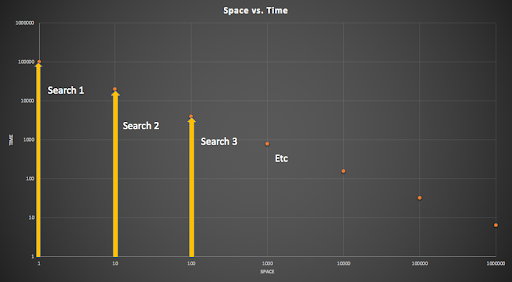This diagram again shows searches increasing from the smaller areas on the left to larger areas on the right, but starting with the longest time period, and reducing as space increases:Decreasing time search with increasing space search3.2 Partition CardinalityAnother observation is that in practice the shorter geohashes are only useful for bootstrapping the system. As more and more data is inserted the longer geohashes will increasingly have sufficient data to satisfy the query, and the shorter geohashes are needed less frequently. So, another way of thinking about the choice of correct partition key is to compute the maximum cardinality. A minimum cardinality of 100,000 is recommended for the partition key. Here’s a table of the cardinality of each geohash length:geohash lengthcardinalitycardinality > 100000132FALSE21024FALSE332768FALSE41048576TRUE533554432TRUE61073741824TRUE734359738368TRUE81.09951E+12TRUEFrom this data, we see that a minimum geohash length of 4 (with an area of 40km^2) is required to satisfy the cardinality requirements. In practice, we could, therefore, make the geohash4 the partition key. At a rate of 220,000 checks per second the partitions could hold 230 days of data before exceeding the maximum partition size threshold. Although we note that the partitions are still technically unbounded, so a composite key and/or TTL (see next) may also be required.3.3 TTLsA refinement of these approaches, which still allows for queries over larger areas, is to use different TTLs for each geohash length. This would work where we have a separate table for each geohash length. The TTLs are set for each table to ensure that the average partition size is under the threshold, the larger areas will have shorter TTLs to limit the partition sizes, while the smaller areas can have much longer TTLs before they get too big (on average, there may still be issues with specific partitions being too big due if data is clumped in a few locations). For the longer geohashes the times are in fact so long that disk space will become the problem well before partition sizes (e.g. geohash5 could retain data for 20 years before the average partition size exceeds 100MB).3.4 Manual ShardingBy default, Cassandra is already “sharded” (the word appears to originate with Shakespeare) by the partition key. I wondered how hard it would be to add manual sharding to Cassandra in a similar way to using a compound partition key (option 1), but where the extra sharding key is computed by the client to ensure that partitions are always close to some fixed size. It turns out that this is possible, and could provide a way to ensure that the system works dynamically irrespective of data rates and clumped data. Here’s a couple of good blogs on sharding in Cassandra (avoid pitfalls in scaling, synthetic sharding).  Finally, Partitions in Cassandra do some take effort to design, so here’s some advice for data modeling recommended practices.Next blog: We add a Dimension of the Third Kind to geohashes—i.e. we go Up and Down!Subscribe to our newsletter below or Follow us on LinkedIn or Twitter to get notified when we add the Third Dimension.