Geospatial Anomaly Detection: Part 1—Massively Scalable Geospatial Anomaly Detection With Apache Kafka® and Apache Cassandra®

Recently we announced that we had reached the end of the Anomalia Machina Blog series, but like Star Trek, the universe just keeps on expanding with endless new versions (> 726 Star Trek episodes and movies in 2016!). I guess this makes this blog an anomaly of sorts.Part 1: The Problem and Initial IdeasThis blog will introduce the problem of Geospatial Anomaly Detection and investigate some initial Cassandra data models based on using latitude and longitude locations.1. Space: The Final FrontierSpace: the final frontier. These are the voyages of the starship Enterprise. Its continuing mission: to explore strange new worlds. To seek out new life and new civilizations. To boldly go where no one has gone before! [Captain Picard]Can you imagine what we’ll find? [Captain Kirk]Alien despots hell-bent on killing us? Deadly spaceborne viruses and bacteria? Incomprehensible cosmic anomalies that could wipe us out in an instant! [Doctor ‘Bones’ McCoy]It’s gonna be so much fun. [Captain Kirk]In recent news (10 April) it is apparent that we don’t need a starship to encounter cosmic anomalies! Just a planet sized telescope (the Event Horizon Telescope) producing data at 64 gigabits per second for 7 days, time stamped with hydrogen maser atomic clocks (which only lose one second every 100 million years), resulting in 5 petabytes of data, transferred on half a ton of hard disks to a single location, and then stitched together on two “correlator” supercomputers and thereafter processed on commodity cloud and GPU computers. After two years, all this data was finally turned into an actual photograph of a real cosmic anomaly, the supermassive black hole at the center of the distant (53 million light-years) M87 galaxy. This black hole definitely counts as a cosmic anomaly—it’s billions of times more massive than the Sun, larger than our solar system, and swallows 90 earths a day. Degree of difficulty?  Like “taking a picture of a doughnut placed on the surface of the moon” (from the earth I guess, as it would be easy to do if you were on the moon next to the doughnut).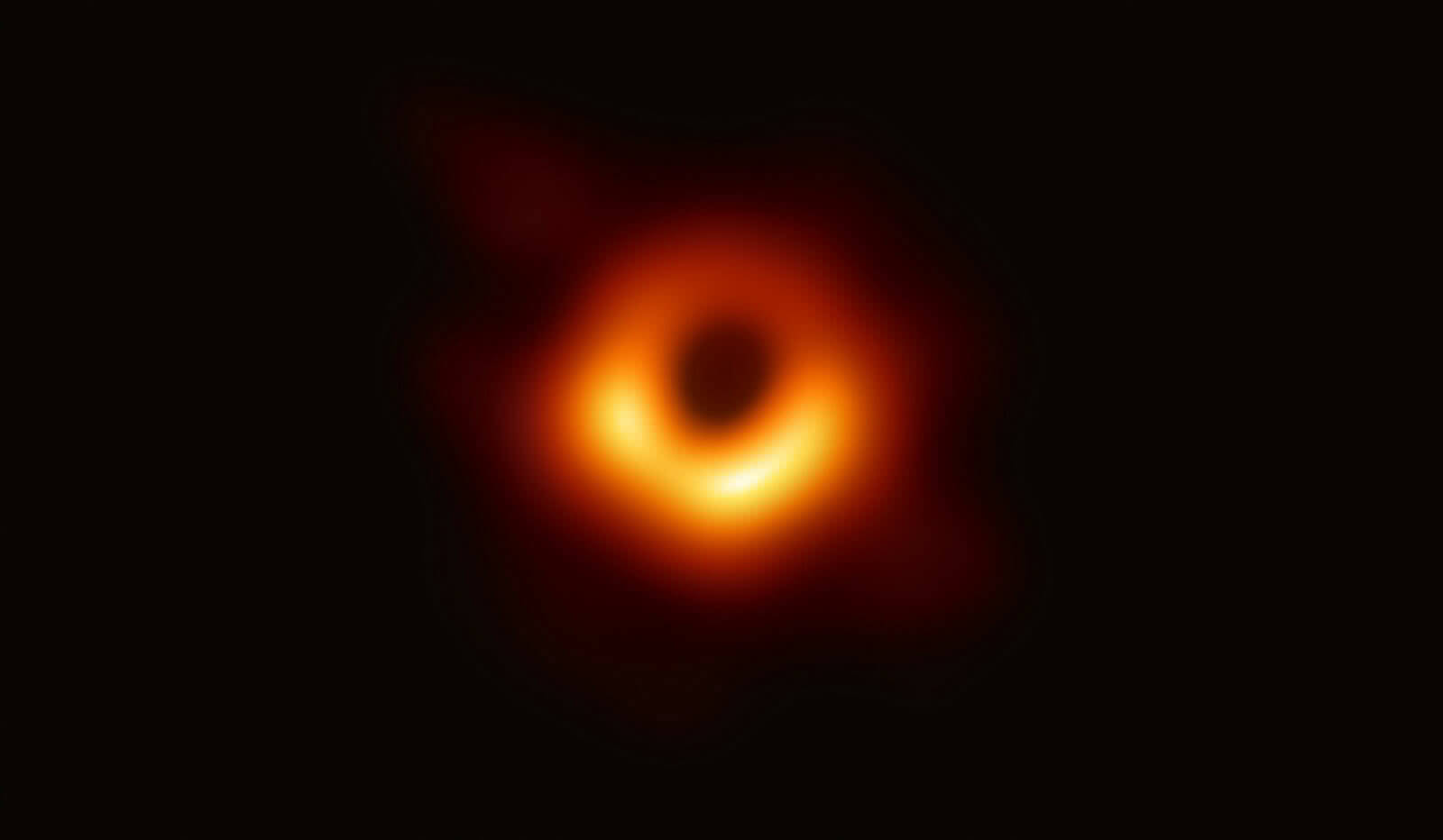The “photo” of the black hole in a galaxy far away  Source:eso.orgAlso in the last month, I started watching the “Project Blue Book”, about the shadowy world of UFO sightings and (maybe) alien encounters which astronomer J. Allen Hynek and his colleague Captain Michael Quinn were tasked to investigate, classify (Hynek’s UFO Classification System has six categories, but only three kinds of “close encounter”), and (officially at least) debunk. Coincidentally, Canberra became the “Drone capital of the world” with the launch of a world-first household drone delivery operation! I predict that the rate of UFO sightings will go up substantially. Time to start plotting those close encounters on a map!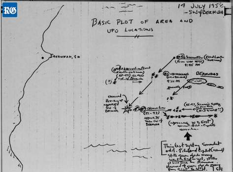A hand-drawn map of close encounters from the Project Blue Book archives.This combination of events was the stimulus for developing an extension of Anomalia Machina, our scalable real-time Anomaly Detection application using Apache Kafka and Cassandra and Kubernetes, for Geospatial Anomaly Detection. My Latin’s not very good, but I think that makes this new series: “Terra Locus Anomalia Machina”. Who knows? Maybe we’ll discover strange anomalies in drone deliveries or even a new type of black hole?!2. The Geospatial Anomaly Detection ProblemSpace is big. Really big. You just won’t believe how vastly, hugely, mind-bogglingly big it is. I mean, you may think it’s a long way down the road to the chemist, but that’s just peanuts to space. Douglas Adams, The Hitchhiker’s Guide to the GalaxySource: ShutterstockHow would a geospatial anomaly detector work? The geospatial problem we want to solve is challenging. Let’s assume that we want to detect anomalies for events that are related in both space and time, but making no assumptions about where in space or how densely clustered they are. The events may be very sparse, spread uniformly across the whole of the planet, or very dense, with many occurring within meters of each other, or a mixture of both.  As a result, we can’t assume a finite number of fixed locations, or a minimum or maximum distance between events as being in “the same location”. We have both location and scale challenges.To usefully represent location we really need some sort of coordinate system and a map with a scale. This map (from “Treasure Island”) is a good start as it has coordinates, scale, and potentially interesting locations marked (e.g. “Bulk of treasure here”):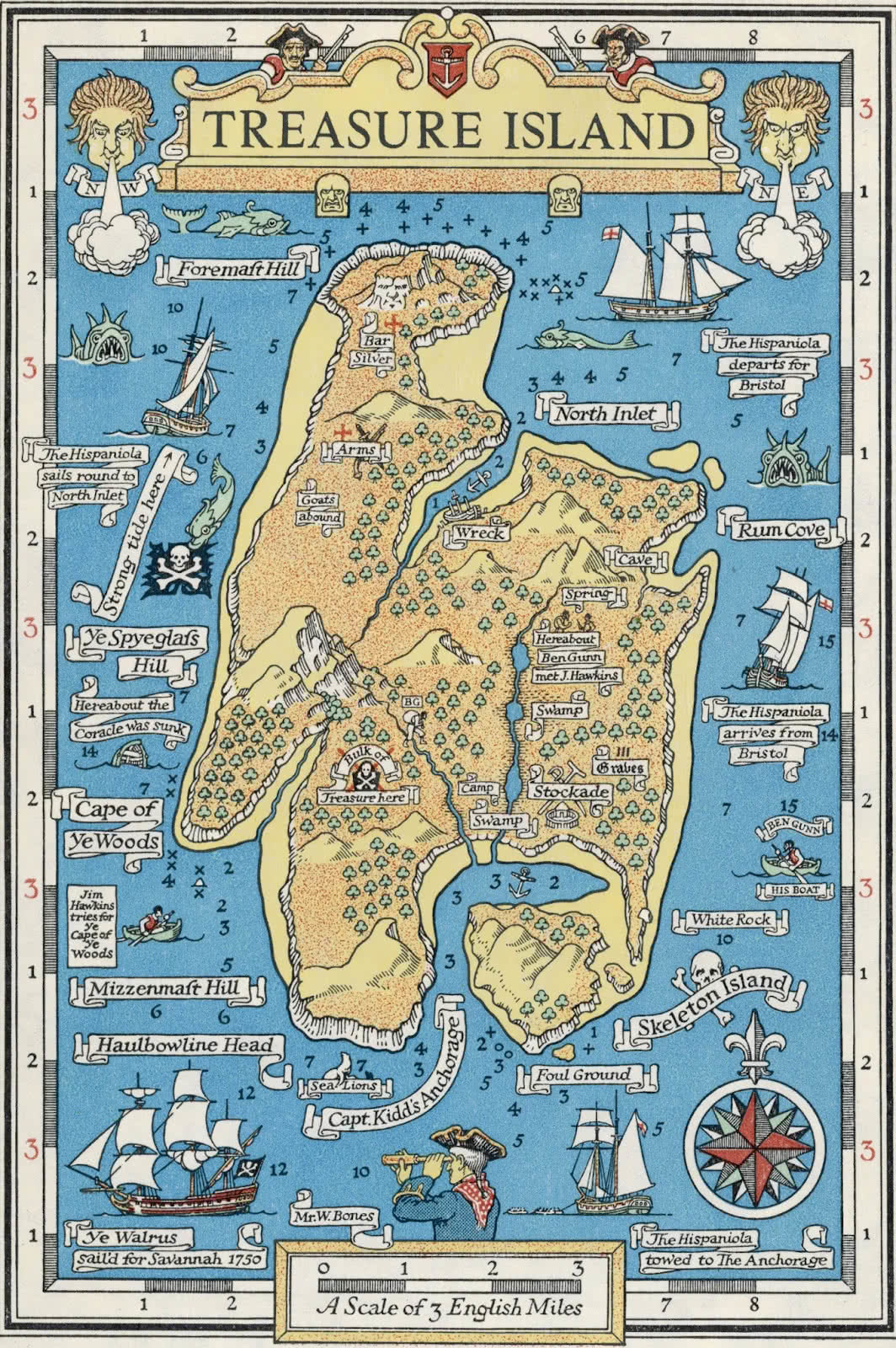Source: openculture.comInstead of a single integer ID (as in the original Anomalia Machina) each event will need location coordinates. We’ll use <latitude, longitude> coordinates, with 10m accuracy (assuming that location is determined by a GPS). Each event also has a single value corresponding to some measurement of interest at that location, e.g. radiation, the number of UFOs detected, the trip length (e.g. of a drone or an Uber etc.). 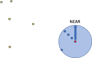We also assume that the events are potentially being produced by a moving device, so events may or may not come from the same exact location, and will definitely come from “new” locations.For each new event coming into the system we want to find the nearest 50 events, in reverse order of time, and then run the anomaly detector over them. This means that nearer events will take precedence over more distant events, even if the more distant events are more recent. 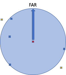It also means that there may not be many events in a particular location (initially, or ever), so the system may have to look an arbitrary distance away to find the nearest 50 events.For example, if the events are sparsely distributed, then the nearest (4 for simplicity) events (blue) are further away from the latest event (red) (we assume these are all on a flat 2d plane with locations as <x,y> cartesian coordinates similar to the Treasure Island Map):If events are denser around a particular location (red) then the (4) nearest events (blue) can be found nearby:Note that as events build up over time there may be “hotspots” where the number of events becomes too high and the older events become irrelevant sooner. We assume that there is a mechanism that can expire events to prevent this becoming a problem. As we will be using Cassandra for data storage, the Cassandra TTL mechanism may be adequate, or we may need a more sophisticated approach to expire events in hotspots faster than other more sparsely populated locations.However, this all depends on how we implement notions of location and proximity. The above examples used a 2d cartesian coordinate system, which looks similar to the Mercator map projection invented in 1569. It’s a cylindrical projection, parallels and meridians are straight and perpendicular to each other which makes the earth look flat and rectangular. However, only sizes along the equator are correct, and it hugely distorts the size of Greenland and Antarctic, but it’s actually very good for navigation, and a variant is widely used for online mapping services.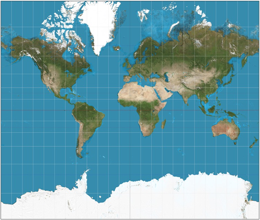Mercator Map – Source: WikipediaSo let’s see how far we get with what has the appearance of a flat earth theory!3. Latitude and LongitudeTo modify the Anomalia Machina application to work with geospatial data we need to (1) modify the Kafka load generator so that it produces data with a geospatial location as well as a value (i.e. we replace the original ID integer key with a geospatial key), (2) write the new data type to Cassandra, and (3) for a given geospatial key, query Cassandra for the nearest 50 events in reverse time order.  The obvious way of representing location is with <latitude, longitude> coordinates, so an initial naive implementation used a pair of decimal <latitude, longitude> values as the geospatial key. But in order to store the new data type, we need to think about what the Casandra table schema should be.As is usual with Cassandra the important question is what should the primary key look like? Cassandra primary keys are made up of two parts: a partition key (simple or compound, which Cassandra uses to determine which node the row is stored on), and zero or more clustering keys (which determine the order of the results). We could use a compound primary key using latitude and longitude, but this would only enable us to look up locations that match exactly with the key. An alternative is to use a different partition key, perhaps the name of the country (assuming we have a simple way of converting <latitude, longitude> into countries, perhaps including oceans to cope with locations at sea), and include <latitude, longitude> as extra columns as follows:Country is the partition key, and time is the clustering key. To find events in an exact location we tried this query:However, this query produces a message saying:Adding “allow filtering” to the query:This works, and returns up to 50 records at the same exact location in reverse time order (Mount Tongariro in New Zealand, perhaps we want to check if it’s about to erupt. This photo is from the last major eruption in 1974 which I remember well as I lived “nearby”, in volcanic scale, less than 100km).Source: GNS ScienceHowever, how does this help us find the 50 nearest events to a location? “Nearest” requires an ability to compute distance. How do you compute the distance between two locations? This would be easy if we go along with the illusion of the above maps, that the earth is flat and we are using <x, y> cartesian coordinates, maybe something like this: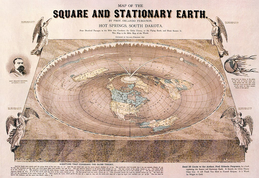Map of Earth made in 1893 by Prof. Orlando Ferguson of Hot Springs, South Dakota  (Source: Wikimedia Commons)It’s time to move beyond a Flat Earth theory (with the associated dangers of falling off the edges and difficulty finding the South Pole). Latitude and Longitude are actually angles (degrees, minutes and seconds) and the earth is really a sphere (approximately). Latitude is degrees North and South of the Equator, Longitude is degrees East and West (of somewhere).(Source: Shutterstock)Degrees, minutes, and seconds, can be converted to/from decimal degrees.  The location of Mount Tongariro in degrees, minutes and seconds is: Latitude: -39° 07′ 60.00″ S Longitude: 175° 38′ 59.99″ E, which in decimal is: <-39.1296, 175.6358>.This diagram shows the decimal degrees (Latitude is φ, Longitude is λ). A latitude of 0 is at the equator. Positive latitudes are north of the equator (90 is the North Pole), negative latitudes are south of the equator (-90 is the South Pole). Latitudes are also called parallels as they are circles parallel to the equator. Positive longitudes are East of an arbitrary line, the “Prime meridian” (which runs through Greenwich in London, with a Longitude of 0), negative longitudes are West of the Prime Meridian. Latitudes range from -180 to 180, and Longitudes range from -90 to 90 degrees.The Mercator map is actually a type of cylindrical projection of a sphere onto a cylinder like this: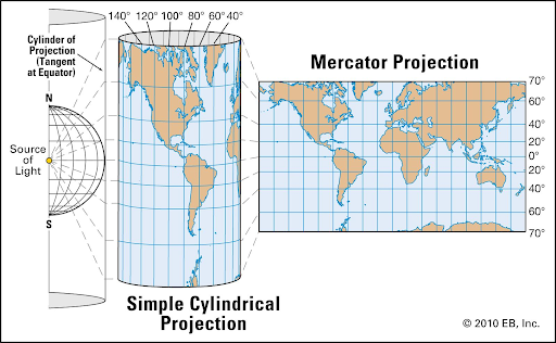(Source: Encyclopedia Britannica)The theoretically correct calculation of distance between two latitude (φ) longitude (λ)  points is non-trivial (the Haversine formula, where r is the radius of the earth, 6371 km, and lat/long angles need to be in radians):But even assuming we can perform this calculation (maybe with a Cassandra UDF), the use of “allow filtering” makes it impractical to use in production as the processing time will continue to grow with partition size.4. Bounding BoxUsing a simpler approximation for distance such as a bounding box calculation means we can then use inequalities (>=, <=) to compute if a point (x2, y2) is approximately within some distance (d) of another point (x, y). This example is for simple (x,y) co-ordinates, as the calculation for latitude and longitude is more complex and requires: converting latitude and longitude to distance (each degree of latitude is approximately 111km and constant, as latitudes are always parallel, but a degree of longitude is 111km at the equator and shrinks to zero at the poles), and careful handling of boundary conditions near the poles (90, and -90 degrees latitude) and near -180 and 180 degrees longitude (the “antimeridian”, which is the basis for the International Date Line, directly opposite the Prime Meridian):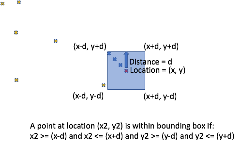Here’s a bounding box query with sides of approximately 100km centred on Mount Tongariro, however, because we still need “allow filtering” it isn’t practical for production:5. IndexingI wondered if indexing the latitude and longitude columns would remove the need for “allow filtering”. Indexing allows rows in Cassandra to be queried by columns other than just those in the partition key. Some Cassandra indexing options include clustering columns, secondary indexes, or SASI indexes.5.1 Clustering ColumnsEven though we are using time as a clustering column already, we can also add latitude and longitude as  clustering columns as follows:However, I discovered that a limitation of clustering columns is that to use an inequality on a clustering column in a “where” clause, all of the preceding columns must have equality relationships, so this isn’t going to work for the bounded box calculation, i.e. this query will work without “allow filtering” (but isn’t correct as it only matches exact latitudes, not ranges):5.2 Secondary IndexesBut what if we add secondary indexes instead? A Cassandra secondary index is an optional index on a column, but should be used with caution.  Let’s create some secondary indexes :However, secondary indexes appear to have the same select query restrictions as Clustering columns, so this didn’t get us any further.5.3 SASIThere is another type of indexing available called SASI (SSTable Attached Secondary Index) which are included in Cassandra by default. SASI supports complex queries more efficiently that the default secondary indexes, including:AND or OR combinations of queries.Wildcard search in string values.Range queries.SASIs are used as follows. Note that you can’t have secondary and SASI indexes on the same column, so you need to drop the secondary indices first.As expected, this did enable more powerful queries, but the complete bounding box query still needed “allow filtering”.  Upon further investigation, the SASI documentation on Compound Queries says that even though “allow filtering” must be used with 2 or more column inequalities, there is actually no filtering taking place, so you could probably use a bounded box query efficiently in practice.  Over the next blog(s) we’ll continue to explore feasible solutions, and finally try some of them out in the Anomalia Machina application, and see how well they work in practice. Given that latitude and longitude locations have proved tricky to use as a basis for proximity queries, we’ll next explore an approach that only needs single column locations and equality in the query: Z-order curves!—more commonly known as Geohashes. These map multidimensional data to one dimension while preserving locality of the data points. And not to be confused with Geohashing which is an (extreme?) sport involving going to random geohash locations and proving that you’ve been there! In the meantime, can you find these geohashes? ‘rchcm5brvd4cn’, ‘sunny’, ‘fur’, ‘reef’, ‘geek’, ‘ebenezer’ and ‘queen’? (Travelling to them is optional).Next Blog: Terra-Locus Anomalia Machina – Part 2: Geohashes, and 3 dimensionsPostscriptIt looks like we’ve been beaten to discovering a new type of cosmic anomaly, as another black hole was recently discovered which is eating its companion star, and spinning so fast it’s pulling space and time around with it (‘Bones’ was correct).