How a 5 node TimescaleDB cluster outperforms 30 Cassandra nodes, with higher inserts, up to 5800x faster queries, 10% the cost, a more flexible data model,
and of course, full SQL.

With its simple data partitioning and distribution architecture, highly tunable consistency settings, and strong cluster management tooling, Cassandra is legendary for its scalability. Developers often forego the expressiveness of SQL for the intoxicating power of being able to add write nodes to a Cassandra cluster with a single command. Moreover, Cassandra’s ability to provide sorted wide rows (more on this later) makes it a compelling use case for a scalable time-series data store.
We’ve already written about how the notion of giving up the structure, maturity, and rich extensibility of PostgreSQL for scalability is a false dilemma. We’ve also pitted TimescaleDB against another popular NoSQL database in our recent benchmarking post about MongoDB. Nonetheless, Cassandra’s ease of use, staying power, and potential to handle time-series data well through its sequentially sorted wide rows make it a natural comparison to TimescaleDB.
In this post, we dig deeper into using Cassandra vs. TimescaleDB for time-series workloads by comparing the scaling patterns, data model complexity, insert rates, read rates, and read throughput of each database. We start by comparing 5 node clusters for each database. Then, we benchmark a few different cluster configurations because the scaling properties of 5 node TimescaleDB and 5 node Cassandra are not perfectly analogous.
Benchmarking Setup
Let’s quickly take stock of the specs we used for these tests:
- 2 remote client machines, both on the same LAN as the databases
- Azure instances: Standard D8s v3 (8 vCPUs, 32 GB memory)
- 5 TimescaleDB nodes, 5/10/30 Cassandra nodes (as noted)
- 4 1-TB disks in a raid0 configuration (EXT4 filesystem)
- Dataset: 4,000 simulated devices generated 10 CPU metrics every 10 seconds for 3 full days (~100M reading intervals, ~1B metrics)
- For TimescaleDB, we set the chunk size to 12 hours, resulting in 6 total chunks (more here)
The Results
Before moving forward, let’s start with a visual preview of how 5 TimescaleDB nodes fare against various sizes of Cassandra clusters:
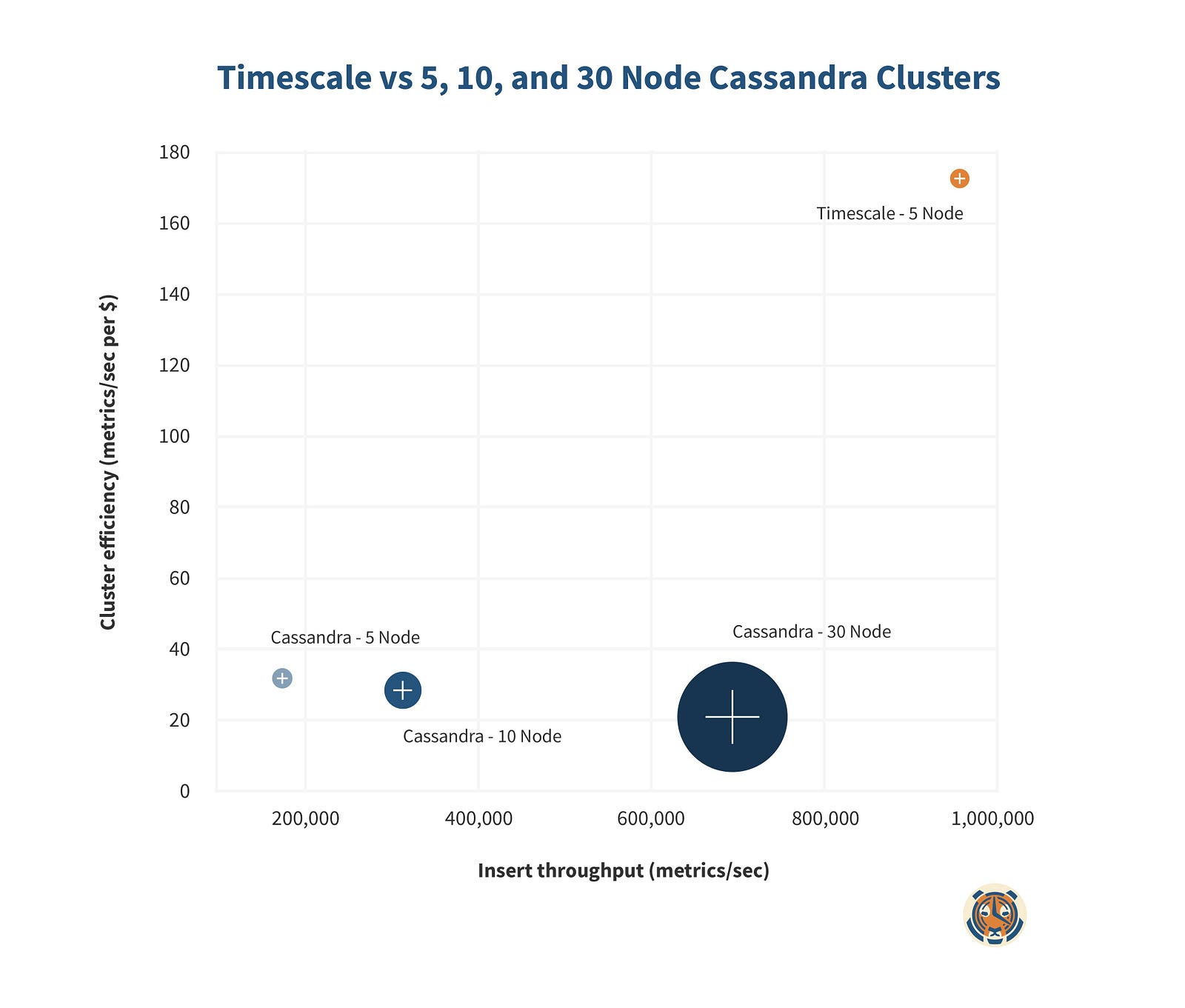
Now, let’s look a bit further into how TimescaleDB and Cassandra achieve scalability.
Scaling with TimescaleDB and Cassandra
Cassandra provides simple scale-out functionality through a combination of its data partitioning, virtual node abstraction, and internode gossip. Adding a node to the cluster redistributes the data in a manner transparent to the client and increases write throughput more-or-less linearly (actually somewhat sub-linear in our tests)¹. Cassandra also provides tunable availability with its replication factor configuration, which determines the number of nodes that have a copy of a given piece of data.
PostgreSQL and TimescaleDB support scaling out reads by way of streaming replication. Each replica node can be used as a read node to increase read throughput. Although PostgreSQL does not natively provide scale-out write functionality, users can often get the additional throughput they need by using RAID disk arrays or leveraging the tablespace functionality provided by PostgreSQL. In addition, unlike PostgreSQL, TimescaleDB allows users to (elastically) assign multiple tablespaces to a single hypertable if desired (e.g., multiple network-attached disks), creating the potential for massively scaling disk throughput on a single TimescaleDB instance. Moreover, as we’ll see, the write performance a single TimescaleDB instance provides for time-series data is quite often more than sufficient for a production workload — and that’s without some of the traditional NoSQL drawbacks that come with Cassandra.
Cassandra shortcomings: poor index support, no JOINs, restrictive query language, no referential integrity
The dead simple scalability of Cassandra does not come without a cost. A number of key features that users of full-SQL databases like TimescaleDB take for granted are either not provided, very cumbersome, or not performant in Cassandra.
Indexes: Unlike traditional SQL databases, Cassandra does not support global indexes, often making it prohibitive to look up or filter data by anything other than the primary or clustering keys. Clustering keys, which we’ll discuss shortly, provide ordering only for a single “row” of data. Cassandra does support secondary indexes, but they are created locally on each node to preserve the scaleable writes of Cassandra. This means that every node must be queried each time an index lookup is performed, often leading to unacceptable performance.
JOINs: Cassandra is not a relational database and does not support natively joining data from two different sources. Users often have to create complex, error prone, and/or tedious client side logic to combine and filter data; indeed, this is what we had to do to get many of our benchmarking queries to be performant. While there are tools available for performing joins in Cassandra, they rely on implementing client-side joins either through heavyweight clients or standalone proxies in front of Cassandra itself.
Query Language: Cassandra’s query language (CQL) lacks the expressiveness of SQL. Much of this has to do with some of the limitations brought on by Cassandra’s architecture. For example, the use of the WHERE clause is limited to primary or clustering keys or fields that have secondary indexes defined on them², otherwise the coordinator would need to retrieve data from every node in the cluster for each query. This is also true of the GROUPBY clause, which was only introduced in Cassandra 3.0. Another significant limitation for many application workflows is that you can only update data using its primary key. These and many other limitations make CQL a poor choice for workloads that require heavy analytical queries or data manipulation on fields beyond the primary and clustering keys.
Referential Integrity: There is no concept of referential integrity in Cassandra. Any constraints that you would typically model as a foreign key relationship in SQL are impossible in Cassandra without writing custom code to enforce them on the client side.
These limitations typically translate to more complicated data models on the server side and much more complicated client-side logic than other databases we’ve benchmarked. We’ll see this on full display in the time-series data model we chose in order to make Cassandra as performant as possible.
Cassandra Data Model
First, a quick note on the origins of our Cassandra data model. In the interest of using a similar foundation for comparing database performance against time series workloads, we forked InfluxDB’s benchmarker for our own internal benchmarks. Their benchmarker comes equipped with a Cassandra time-series data model. We adopted their model largely as is, as we found their reasoning sufficiently compelling and aligned with canonical approaches to time-series data in Cassandra.
That being said, we definitely do not consider ourselves Cassandra gurus, so we’re all ears if the community has suggestions on a better model that would improve our benchmarks. We plan to release our benchmarker in the coming weeks, and we’re eager to hear from any experts on various databases who would like to weigh in and help make our benchmarks more robust in general.
Cassandra is a column family store. Data for a column family, which is roughly analogous to a table in relational databases, is stored as a set of unique keys. Each of these keys maps to a set of columns which each contain the values for a particular data entry. These key->column-set tuples are called “rows” (but should not be confused with rows in a relational database).
In Cassandra, data is partitioned across nodes based on the column family key (called the primary or partition key). Additionally, Cassandra allows for compound primary keys, where the first key in the key definition is the primary/partition key, and any additional keys are known as clustering keys. These clustering keys specify columns on which to sort the data for each row.
Let’s take a look at how this plays out with the dataset we use for our benchmarks. We simulate a devops monitoring use case where 4,000 unique hosts report 10 CPU metrics every 10 seconds over the course of 3 days, resulting in a 100 million row dataset.
In our Cassandra model, this translates to us creating a column family like this:
CREATE TABLE measurements (
series_id text,
timestamp_ns bigint,
value double,
PRIMARY KEY(series_id, timestamp_ns));
The primary key, series_id, is a combination of the host, day, and metric type in the format hostname#metric_type#day. This allows us to get around some of the query limitations of Cassandra discussed above, particularly the weak support for joins, indexes, and server side rollups. By encoding the host, metric type, and day into the primary key, we can quickly and easily access the subset of data we need and execute any further filtering, aggregation, and grouping more performantly on the client side.
We use timestamp_ns as our clustering key, which means that data for each row is ordered by timestamp as we insert it, providing optimal time range lookups. This is what a row of 3 values of the cpu_guest metric for a given host on a given day would look like:
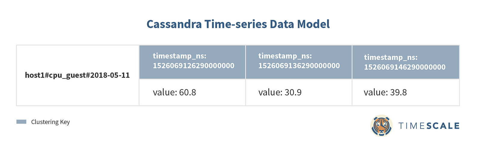
This is what we meant when we mentioned the wide row approach earlier. Each row contains multiple columns, which are themselves sets of key-value pairs. The number of columns for a given row grows as we insert more readings corresponding to that row’s partition key. The columns are clustered by their timestamp, guaranteeing that each row will point to a sequentially sorted set of columns.
This ordered data is passed down to our custom client, which maintains a fairly involved client-side index to perform the filtering and aggregation that is not supported in a performant manner by Cassandra’s secondary indexes. We maintain a data structure that essentially duplicates Cassandra’s primary key->metrics mapping and performs filtering and aggregations as we add data from our Cassandra queries. The aggregations and rollups we do on the client side are very simple (min, max, avg, groupby, etc.), so the vast majority of the query time remains at the database level. (In other words, the client-side index works, but also takes a lot more work.)
Insert Performance
Unlike TimescaleDB, Cassandra does not work well with large batch inserts. In fact, batching as a performance optimization is explicitly discouraged due to bottlenecks on the coordinator node if the transaction hits many partitions. Cassandra’s default maximum batch size setting is very small at 5KB. Nonetheless, we found that a small amount of batching (batches of 100) actually did help significantly with insert throughput for our dataset, so we used a batch size of 100 for our benchmarks.
To give Cassandra a fair shake against TimescaleDB, which allows for far larger batch sizes (we use 10,000 for our benchmarks), we ramped up the number of concurrent workers writing to Cassandra. While we used just 8 concurrent workers to maximize our write throughput on TimescaleDB, we used 1,800 concurrent workers (spread across multiple client machines) to max out our Cassandra throughput. We tested worker counts from 1 up to 1,800 before settling on 1,800 as the optimal number of workers for maximizing write throughput. Any number of workers above that caused unpredictable server side timeouts and negligible gains (in other words, the tradeoff of latency for throughput became unacceptable).
To avoid client-side bottlenecks (e.g., with data serialization, the client-side index, or network overhead), we used 2 client VMs, each using our Golang benchmarker with 900 goroutines writing concurrently. We attempted to get more throughput by spreading the client load across even more VMs, but we found no improvements beyond 2 boxes.
Since writes are sharded across nodes in Cassandra, its replication and consistency profile is a bit different than that of TimescaleDB. TimescaleDB writes all data to a single primary node which then replicates that data to any connected replicas through streaming replication. Cassandra, on the other hand, shards the writes across the cluster, so no single replica stores all the cluster’s data. Instead, you define the replication factor for a given keyspace, which determines the number of nodes that will have a copy of each data item. You can further control the consistency of each write transaction on the client side by specifying how many nodes the client waits for the data to be written to. PostgreSQL and TimescaleDB similarly offer tunable consistency.
Given these significant differences, it’s difficult to achieve a truly apples-to-apples comparison of a 5 node TimescaleDB cluster vs. a 5 node Cassandra cluster. We decided on comparing a TimescaleDB cluster with 1 primary and 4 read replicas, synchronous replication, and a consistency level of ANY 1 against a 5 node Cassandra cluster with Replication Factor set to 2 and a consistency level of ONE. In both cases, clients will wait on data to be copied to 1 replica. Eventually data will be copied to 2 nodes in the case of Cassandra, while data will be copied to all nodes in the case of TimescaleDB.
In theory, then, Cassandra should have an advantage in insert performance since writes will be sharded across multiple nodes. On the read side, TimescaleDB should have a small advantage for very hot sets of keys (given they may be more widely replicated), but the total read throughput of the two should be theoretically comparable.
In practice, however, we find that TimescaleDB has an advantage over Cassandra in both reads and writes, and it’s large.
Let’s take a look at the insert rates for each cluster:
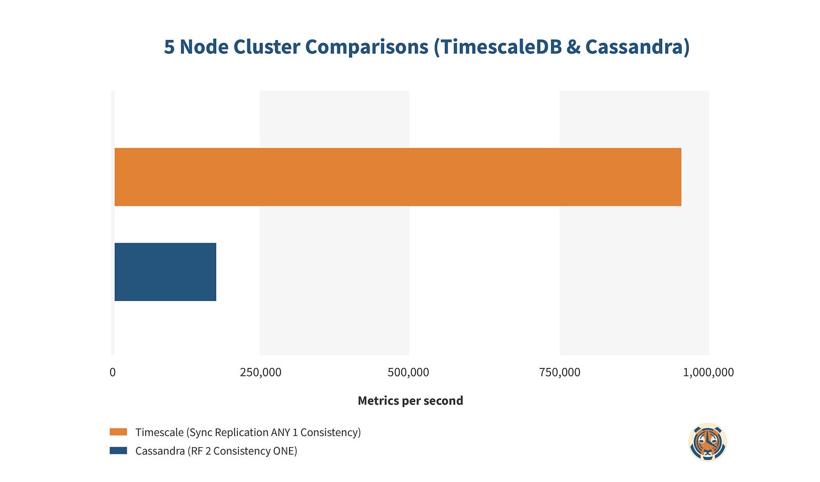
Despite Cassandra having the theoretical advantage of sharded writes, TimescaleDB exhibits 5.4x higher write performance than Cassandra. That actually understates the performance difference. Since TimescaleDB gets no write performance gains from adding extra nodes, we really only need a 3 node TimescaleDB cluster to achieve the same availability and write performance as our Cassandra cluster, making the real TimescaleDB performance multiplier closer to 7.6x.
This assumes that Cassandra scales perfectly linearly, which turns out to not quite be the case in our experience. We increased our Cassandra cluster to 10 then 30 nodes while keeping TimescaleDB at a cool 5 nodes:
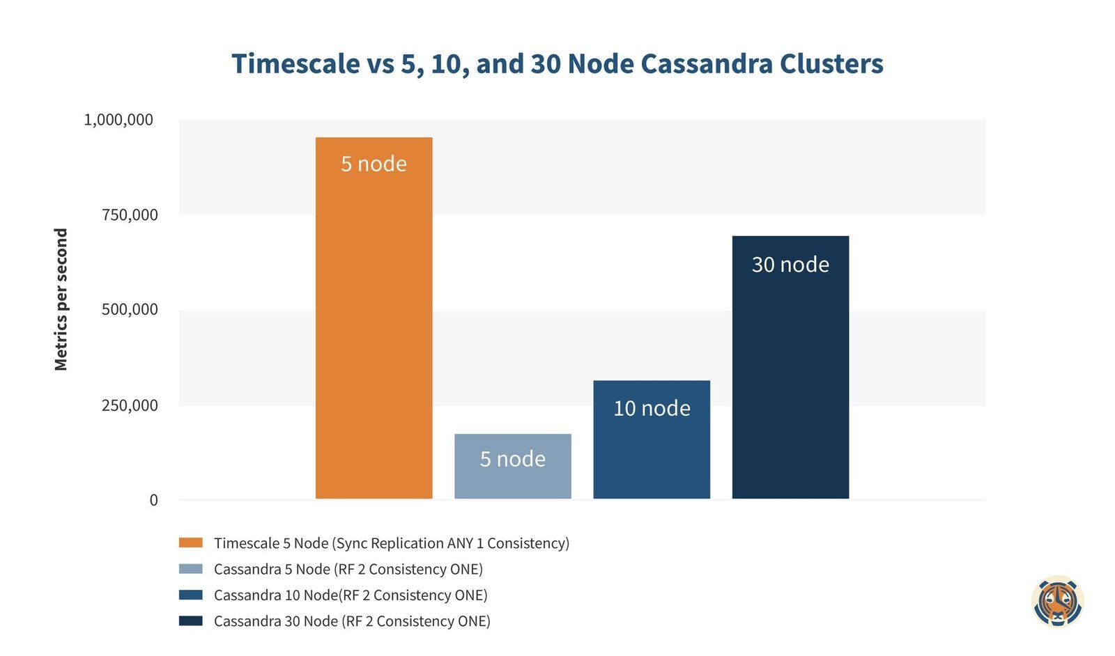
Even a 30 node Cassandra cluster performs nearly 27% slower for inserts against a single TimescaleDB primary. With 3 TimescaleDB nodes — the maximum with TimescaleDB needed to provide the same availability as 30 node Cassandra with a Replication Factor of 2 — we now see that Cassandra needs well over 10x (probably closer to 15x) the resources as TimescaleDB to achieve similar write rates.
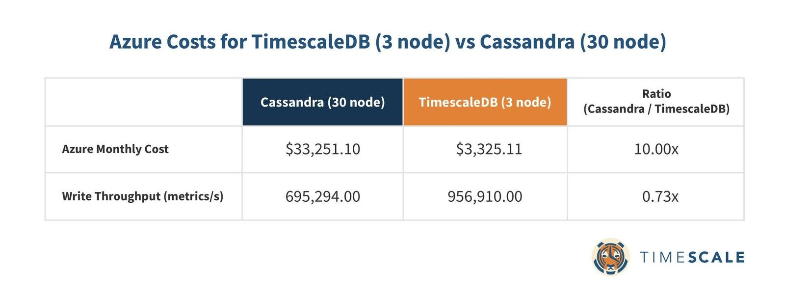
For each node in these benchmarks, we paid for an Azure D8s v3 VM ($616.85/month) as well as 4 attached 1TB SSDs ($491.52/month). The minimum number of TimescaleDB nodes needed to achieve its write throughput and availability in the above chart is 3 ($3,325.11/month), while the minimum number of Cassandra nodes required to achieve its highest write throughput and availability in the above chart is 30 ($33,251.10/month). In other words, we paid $29,925.99 more for Cassandra to get 73% as much write throughput as TimescaleDB.
Put another way, TimescaleDB exhibits higher inserts at 10% of the cost of Cassandra.
Query Performance
Cassandra is admittedly less celebrated than SQL databases for its strength with analytical queries, but we felt it was worth diving into a few types of queries that come up frequently with time-series datasets. For all queries, we used 4 concurrent clients per node per query. We measured both the mean query times and the total read throughput in queries per second.
Simple Rollups: TimescaleDB competitive (up to 4x faster)
We’ll start with the mean query time on a few single rollup (i.e., groupby) queries on time. We ran these queries in 1000 different permutations (i.e., random time ranges and hosts).
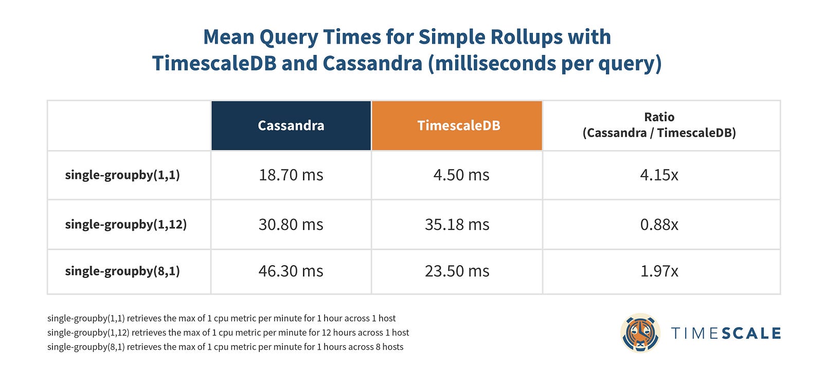
Cassandra holds its own here, but TimescaleDB is markedly better on 2 of the 3 simple rollup types and very competitive on the other. Even in simple time rollup queries where Cassandra’s clustering keys should really shine, TimescaleDB’s hypertables outperform.
Deducing the total read throughput of each database is fairly intuitive from the above chart, but let’s take a look at the recorded QPS of each queryset just to make sure there are no surprises:
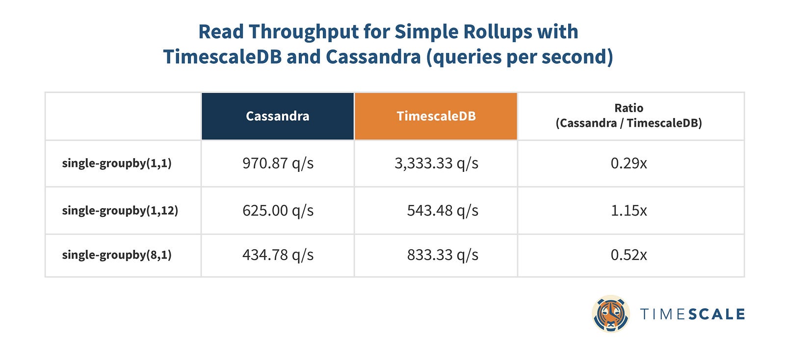
When it comes to read throughput, TimescaleDB maintains its markedly better performance here.
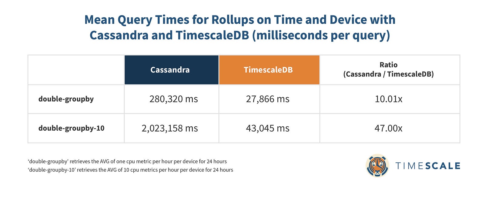
Rollups on Time and Device: TimescaleDB 10x-47x faster
Bringing multiple rollups (across both time and device) into the mix starts to make both databases sweat, but TimescaleDB has a huge advantage over Cassandra, especially when it comes to rolling up multiple metrics. Given the lengthy mean read times here, we only ran 100 for each query type.
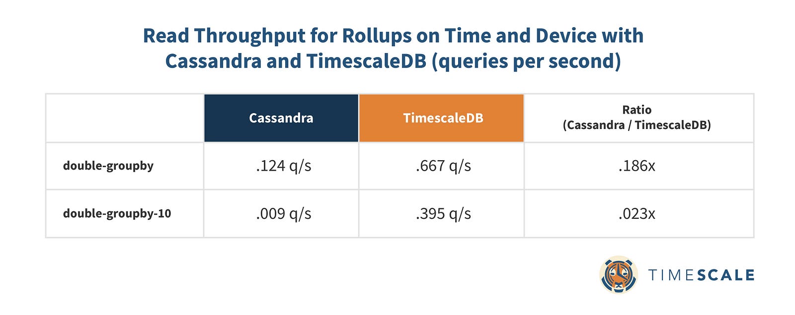
We see a similar story for read throughput:
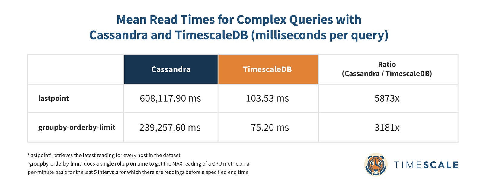
Complex Analytical Queries: TimescaleDB 3100x-5800x faster
We also took a look at 2 slightly more complex queries that you commonly encounter in time-series analysis.
The first (‘lastpoint’) is a query that retrieves the latest reading for every host in the dataset, even if you don’t a priori know when it last communicated with the database³.
The second (‘groupby-orderby-limit’) does a single rollup on time to get the MAX reading of a CPU metric on a per-minute basis for the last 5 intervals for which there are readings before a specified end time⁴.
Each queryset was run 100 times.
And the read throughput:
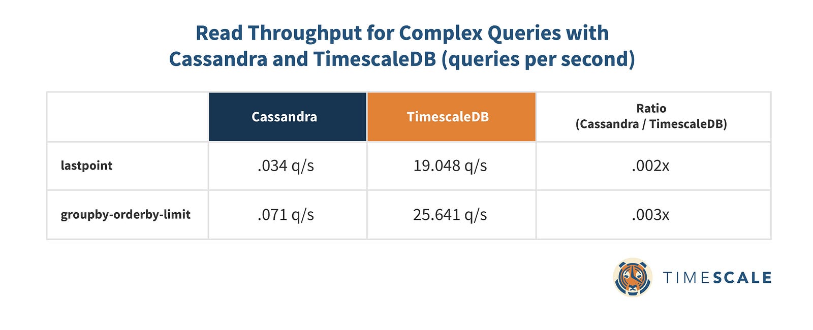
For these queries, Cassandra is clearly not the right tool for the job. TimescaleDB can easily leverage hypertables to narrow the search space to a single chunk, using a per-chunk index on host and time to gather our data from there. Our multi-part primary key on Cassandra, on the other hand, provides no guarantee that all of the data in a given time range will even be on a single node. In practice, for queries like this that touch every host tag in the data set, we end up scanning most, if not all, of the nodes in a cluster and grouping on the client side.
Conclusion
As we see, 5 TimescaleDB nodes outperform a 30 node Cassandra cluster, with higher inserts, up to 5800x faster queries, 10% the cost, a much more flexible data model, and full SQL.
Cassandra’s turnkey write scalability comes at a steep cost. For all but the simplest rollup queries, our benchmarks show TimescaleDB with a large advantage, with average query times anywhere from 10 to 5,873 times faster for common time-series queries. While Cassandra’s clustered wide rows provide good performance for querying data for a single key, it quickly degrades for complex queries involving multiple rollups across many rows.
Additionally, while Cassandra makes it easy to add nodes to increase write throughput, it turns out you often just don’t need to do that for TimescaleDB. With 10–15x the write throughput of Cassandra, a single TimescaleDB node with a couple of replicas for high availability is more than adequate for dealing with workloads that would require a 30+ node fleet of Cassandra instances to handle.
However, Cassandra’s scaling model does offer nearly limitless storage since adding more storage capacity is as simple as adding another node to the cluster. A single instance of TimescaleDB currently tops out around 50–100TB. If you need to store petabyte scale data and can’t take advantage of retention policies or rollups, then massively clustered Cassandra might be the solution for you. However, we’re actively working on a clustered version of TimescaleDB that will similarly allow users to add nodes to increase write throughput and storage capacity — so please stay tuned for more details.
Also, we don’t claim to be Cassandra experts. We’ve tried to be as open as we can about our data models, configurations, and methodologies so readers can raise any concerns they may have about our benchmarks and help us make them as accurate as possible.
As a time-series database company we’ll always be quite interested in evaluating the performance of other solutions. Cassandra was a pleasure to work with in terms of scaling out write throughput. But attaining that at the cost of per-node performance, the vibrant PostgreSQL ecosystem, and the expressiveness of full SQL simply does not seem worth it.