
In this blog post, we’ll dig into the brand new materialized view feature of Cassandra 3.0. We’ll see how it is implemented internally, how you should use it to get the most of its performance and which caveats to avoid.
For the remaining of this post Cassandra == Apache Cassandra™
Being an evangelist for Apache Cassandra for more than a year, I’ve spent my time talking about the technology and especially providing advices and best practices for data modeling.
One of the key point with Cassandra data model is denormalization, aka duplicate your data for faster access. You’re trading disk space for read latency.
If your data is immutable by nature (like time series data/sensor data) you’re good to go and it should work like a charm.
However, mutable data that need to be denormalized are always a paint point. Generally people end up with the following strategies:
- denormalize immutable data
- for mutable data, either:
- accept to normalize them and pay the price of extra-reads but don’t care about mutation
- denormalize but pay the price for read-before-write and manual handling of updates
- since denormalization is required most of the time for different read patterns, you can rely on a 3rd party indexing solution (like Datastax Enterprise Search or Stratio Lucene-based secondary index or more recently the SASI secondary index) for the job
Both solutions for mutable data are far from ideal because it incurs much overhead for developers (extra-read or sync updated data on the client side)
The materialized views have been designed to alleviate the pain for developers, although it does not magically solve all the overhead of denormalization.
Below is the syntax to create a materialized view:
CREATE MATERIALIZED VIEW [IF NOT EXISTS] keyspace_name.view_name AS
SELECT column1, column2, ...
FROM keyspace_name.base_table_name
WHERE column1 IS NOT NULL AND column2 IS NOT NULL ...
PRIMARY KEY(column1, column2, ...)
At first view, it is obvious that the materialized view needs a base table. A materialized view, conceptually, is just another way to present the data of the base table, with a different primary key for a different access pattern.
The alert reader should remark the clause WHERE column1 IS NOT NULL AND column2 IS NOT NULL …. This clause guarantees that all columns that will be used as primary key for the view are not null, of course.
Some notes on the constraints that apply to materialized views creation:
- The AS SELECT column1, column2, … clause lets you pick which columns of the base table you want to duplicate into the view. For now, you should pick at least all columns of the base table that are part of it’s primary key
- The WHERE column1 IS NOT NULL AND column2 IS NOT NULL … clause guarantees that the primary key of the view has no null column
- The PRIMARY KEY(column1, column2, …) clause should contain all primary key columns of the base table, plus at most one column that is NOT part of the base table’s primary key.The order of the columns in the primary key does not matter, which allows us to access data by different patterns
An example is worth a thousand words:
CREATE TABLE user(
   id int PRIMARY KEY,
   login text,
   firstname text,
   lastname text,
   country text,
   gender int
);
CREATE MATERIALIZED VIEW user_by_country
AS SELECT *  //denormalize ALL columns
FROM user
WHERE country IS NOT NULL AND id IS NOT NULL
PRIMARY KEY(country, id);
INSERT INTO user(id,login,firstname,lastname,country) VALUES(1, 'jdoe', 'John', 'DOE', 'US');
INSERT INTO user(id,login,firstname,lastname,country) VALUES(2, 'hsue', 'Helen', 'SUE', 'US');
INSERT INTO user(id,login,firstname,lastname,country) VALUES(3, 'rsmith', 'Richard', 'SMITH', 'UK');
INSERT INTO user(id,login,firstname,lastname,country) VALUES(4, 'doanduyhai', 'DuyHai', 'DOAN', 'FR');
SELECT * FROM user_by_country;
 country | id | firstname | lastname | login
---------+----+-----------+----------+------------
      FR |  4 |    DuyHai |     DOAN | doanduyhai
      US |  1 |      John |      DOE |       jdoe
      US |  2 |     Helen |      SUE |       hsue
      UK |  3 |   Richard |    SMITH |     rsmith
SELECT * FROM user_by_country WHERE country='US';
 country | id | firstname | lastname | login
---------+----+-----------+----------+-------
      US |  1 |      John |      DOE |  jdoe
      US |  2 |     Helen |      SUE |  hsue
In the above example, we want to find users by their country code, thus the WHERE country IS NOT NULL clause. We also need to include the primary key of the original table (AND id IS NOT NULL)
The primary key of the view is composed of the country as partition key. Since there can be many users in the same country, we need to add the user id as clustering column to distinguish them.
The rationale for the clause WHERE xxx IS NOT NULL is to guarantee that null values in the base table will NOT be denormalized to the view. For example, an user who did not set his country won’t be copied to the view, mainly because SELECT * FROM user_by_country WHERE country = null doesn’t make sense since country is part of the primary key. Also, in the future, you may be able to use other clauses than the IS NOT NULL, mainly using User Defined Functions to filter data to be denormalized.
The rationale for the constraint (all primary key columns of the base table, plus at most one column that is NOT part of the base table’s primary key) is to avoid null value for the primary key.
Example:
CREATE MATERIALIZED VIEW user_by_country_and_gender
AS SELECT *  //denormalize ALL columns
FROM user
WHERE country IS NOT NULL AND gender IS NOT NULL AND id IS NOT NULL
PRIMARY KEY((country, gender),id)
INSERT INTO user(id,login,firstname,lastname,country,gender) VALUES(100,'nowhere','Ian','NOWHERE',null,1);
INSERT INTO user(id,login,firstname,lastname,country,gender) VALUES(100,'nosex','Jean','NOSEX','USA',null);
With the above example, both users ‘nowhere‘ and ‘nosex‘ cannot be denormalized into the view because at least one column that is part of the view primary key is null.
In the future, null values may be considered as yet-another-value and this restriction may be lifted to allow more than 1 non primary key column of the base table to be used as key for the view.
A Materialized View update steps
Below is the sequence of operations when data are inserted/updated/deleted in the base table
- If the system property cassandra.mv_enable_coordinator_batchlog is set, the coordinator will create a batchlog for the operation
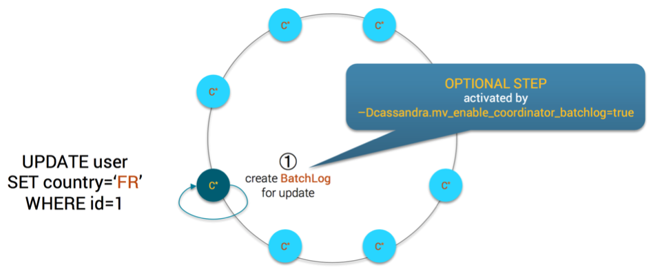
MV Step1
- the coordinator sends the mutation to all replicas and will wait for as many acknowledgement(s) as requested by Consistency Level
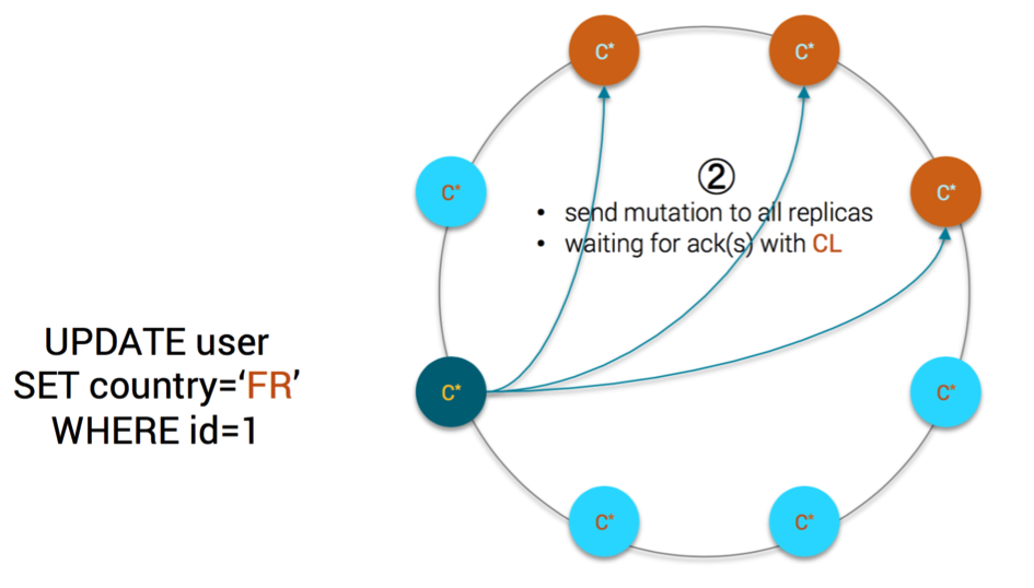
MV Step2
- each replica is acquiring a local lock on the partition to be
inserted/updated/deleted in the base table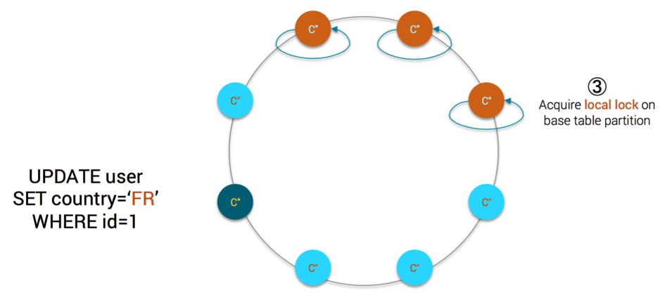
MV Step3
- each replica is performing a local read on the partition of the base table
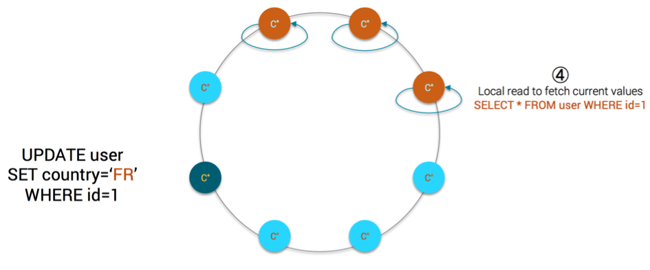
MV Step4
- each replica creates a local batchlog with the following statements:
- DELETE FROM user_by_country WHERE country = ‘old_value’
- INSERT INTO user_by_country(country, id, …) VALUES(‘FR’, 1, …)
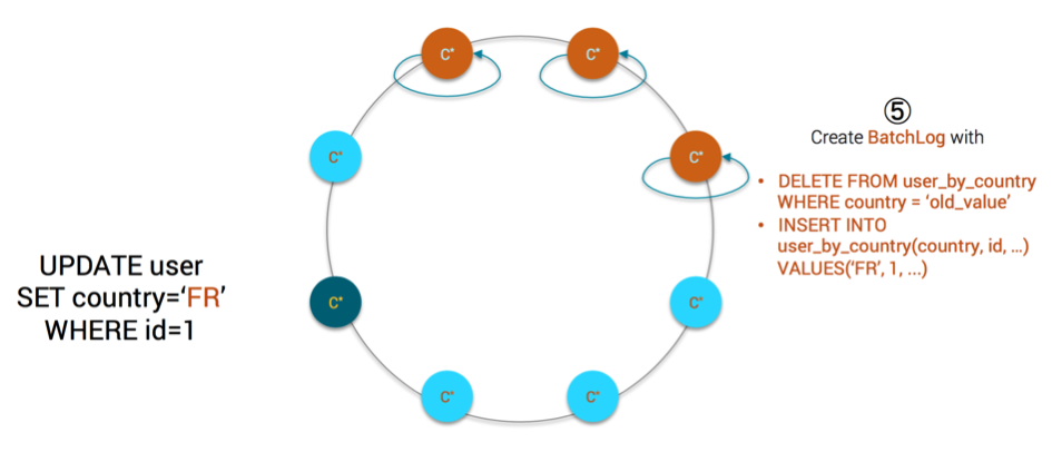
MV Step5
- each replica executes the batchlog asynchronously. For each statement in the batchlog, it is executed against a paired view replica (explained later below) using CL = ONE
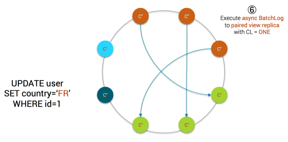
MV Step6
- each replica applies the mutation on the base table locally
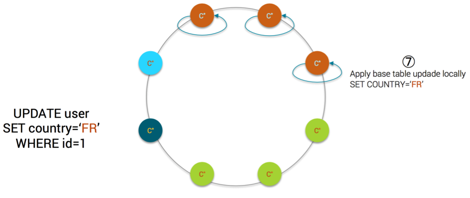
MV Step7
- each replica releases the local lock on the partition of the base table
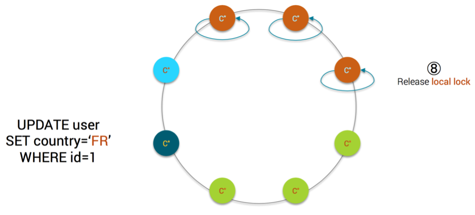
MV Step8
- If the local mutation is successful, each replica sends an acknowledgement back to the coordinator
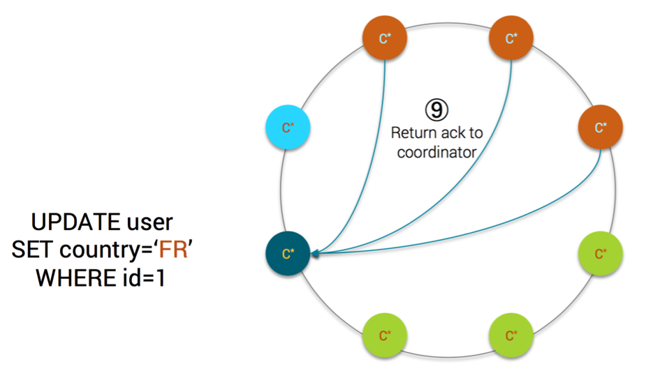
MV Step9
- if as many acknowledgement(s) as Consistency Level are received by the coordinator, the client is acknowledged that the mutation is successful
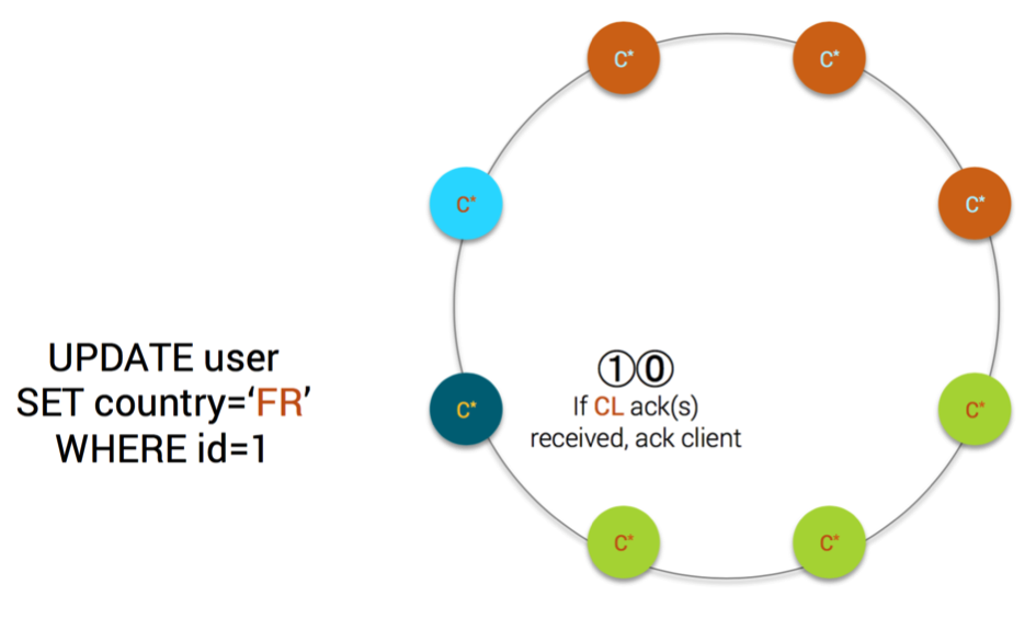
MV Step10
- optionally, if the system property cassandra.mv_enable_coordinator_batchlog is set and if a QUORUM of acknowledgements are received by the coordinator, the coordinator-level batchlog is removed
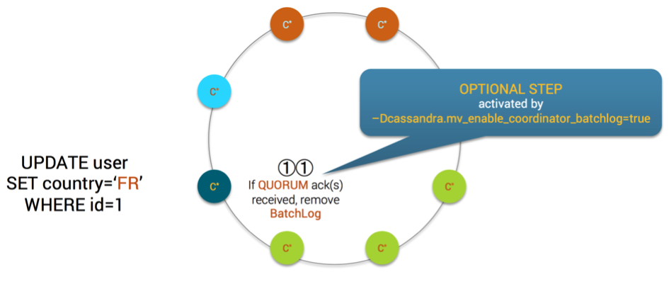
MV Step11
B Paired view replica definition
Before explaining in detail the rationale of some technical steps, let’s define what is a paired view replica. Below is the formal definition in the source code:
The view natural endpoint is the endpoint which has the same cardinality as this node in the replication factor.
The cardinality is the number at which this node would store a piece of data, given the change in replication factor.
If the keyspace’s replication strategy is a NetworkTopologyStrategy, we filter the ring to contain only nodes in the local datacenter when calculating cardinality.
For example, if we have the following ring:
- A, T1 -> B, T2 -> C, T3 -> A
For the token T1, at RF=1, A would be included, so A’s cardinality for T1 is 1.
For the token T1, at RF=2, B would be included, so B’s cardinality for token T1 is 2.
For the token T3, at RF=2, A would be included, so A’s cardinality for T3 is 2.For a view whose base token is T1 and whose view token is T3, the pairings between the nodes would be:
- A writes to C (A’s cardinality is 1 for T1, and C’s cardinality is 1 for T3)
- B writes to A (B’s cardinality is 2 for T1, and A’s cardinality is 2 for T3)
- C writes to B (C’s cardinality is 3 for T1, and B’s cardinality is 3 for T3)
C Local lock on base table partition
The reader should wonder why each replica needs to acquire a local lock on the base table partition since locking is expensive. The reason of this lock is to guarantee view update consistency in case of concurrent updates on the base table partition.
Let’s say we have 2 concurrent updates on an user (id=1) whose original country is UK:
- UPDATE … SET country=’US’ WHERE id=1
- UPDATE … SET country=’FR’ WHERE id=1
Without the local lock, we’ll have interleaved mutations for the view
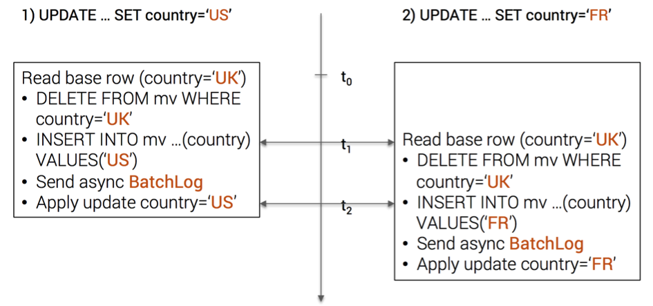
Interleaved Mutations
The user (id=1) now has 2 entries in the view table (country=’US‘ and country=’FR‘)
This issue is fixed with the local lock

Serialized Mutations
Indeed, it is necessary that the sequence of operations 1) read base table data 2) remove view old partition 3) insert view new partition is executed atomically, thus the need of locking
D Local batchlog for view asynchronous update
The local batchlog created on each replica for view update guarantees that, even in case of failure (because a view replica is temporarily down for example), the view update will eventually be committed.
The consistency level ONE is used because each base table replica is responsible for the update of its paired view replica, thus consistency level ONE is sufficient.
Furthermore, the update of each paired view replica is performed asynchronously, e.g. the replica will not block and wait for an acknowledgement before processing to base table mutation. The local batchlog guarantees automatic retries in case of error.
E View data consistency level
The consistency level requested by the client on the base table is respected, e.g. if QUORUM is required (RF=3), the coordinator will acknowledge a successful write only if it receives 2 acks from base table replicas. In this case, the client is sure that the base table update is made durable on at least 2 replicas out of 3.
The consistency guarantee is weaker for view table. With the above example, we only have the guarantee that the view will be updated eventually on at least 2 view replicas out of 3.
The main difference in term of guarantee compared to base table lies in the eventually (asynchronous local batchlog). At the time the coordinator receives 2 acks from base table replicas, we are not sure that the view has been updated on at least 2 replicas.
F Coordinator batchlog
The system property cassandra.mv_enable_coordinator_batchlog only helps in edge cases. Let’s consider below an example of such edge-case:
- coordinator receives update, starts sending to base replicas
- coordinator sends update to one base replica
- base replica receives the update and starts to process
- coordinator dies before update is sent to any other base replica
- base replica sends update to view replica through async local batch
- base replica dies and cannot be brought back up
- view replica processes update
It’s very unlikely for all of those to happen, so protecting against that case while paying such a high penalty with coordinator batchlog doesn’t make sense in the general case and the parameter cassandra.mv_enable_coordinator_batchlog is disabled by default.
Compared to a normal mutation, a mutation on a base table having materialized views will incur the following extra costs:
- local lock on base table partition
- local read-before-write on base table partition
- local batchlog for materialized view
- optionally, coordinator batchlog
In practice, most of the performance hits are incurred by the local read-before-write but this cost is only paid once and does not depends on the number of views associated with the table.
However, increasing the number of views will have an impact on the cluster-wide write throughput because for each base table update, you’ll add an extra (DELETE + INSERT) * nb_of_views load to the cluster.
That being said, it does not make sense to compare raw write throughput between a normal table and a table having views. It’s more sensible to compare write throughput between a manually denormalized table (using logged batch client-side) and the same table using materialized views. In this case, automatic server-side denormalization with materialized views clearly wins because:
- it saves network traffic for read-before-write
- it saves network traffic for logged batch of denormalized table mutations
- it removes the pain for the developer from having to keep denormalized tables synced with base tables
Another performance consideration worth mentioning is hot-spot. Similar to manual denormalization, if your view partition key is chosen poorly, you’ll end up with hot spots in your cluster. A simple example with our user table is to create a materialized view user_by_gender
// THIS IS AN ANTI-PATTERN !!!!
CREATE MATERIALIZED VIEW user_by_gender
AS SELECT * FROM user
WHERE id IS NOT NULL AND gender IS NOT NULL
PRIMARY KEY(gender, id)
With the above view, all users will end up in only 2 partitions: MALE & FEMALE. You certainly don’t want such hot-spots in your cluster.
Now, how do materialized views compare to secondary index for read performance ?
Depending on the implementation of your secondary index, the read performance may vary. If the implementation performs a scatter-gather operation, the read performance will be closely bound to the number of nodes in the datacenter/cluster.
Even with a smart implementation of secondary index like SASI that does not scan all the nodes, a read operation always consist of 2 different read paths hitting disk:
- read the index on disk to find relevant primary keys
- read the source data from C*
That being said, it’s pretty obvious that materialized views will give you better read performance since the read is straight-forward and done in 1 step. The idea is that you pay the cost at write time for a gain at read time.
Still, materialized views loose against advanced secondary index implementation in term of querying because only exact match is allowed, ranged scans (give me user where country is between ‘UK’ and ‘US’) will ruin your read performance.
We do not forget our ops friends and in this chapter, we discuss the impact of having materialized views in term of operations.
Repair & hints :
- it is possible to repair a view independently from its base table
- if the base table is repaired, the view will also be repaired thanks to the mutation-based repair (repair that goes through write path, unlike normal repair)
- read-repair on views behave like normal read-repair
- read-repair on base table will also repair views
- hints replay on base table will trigger mutations on associated views
Schema :
- materialized views can be tuned as any standard table (compaction, compression, …). Use the ALTER MATERIALIZED VIEW command
- you cannot drop a column from based table that is used by a materialized view, even if this column is not part of the view primary key
- you can add a new column to the base table, its initial value will be set to null in associated views
- you cannot drop the base table, you have to drop all associated views first
This section is purely technical for those who want to understand the deep internals. You can safely skip it
During the developement of materialized view some issues arose with tombstones and view timestamps. Let’s take this example:
CREATE TABLE base (a int, b int, c int, PRIMARY KEY (a));
CREATE MATERIALIZED VIEW view AS
    SELECT * FROM base
    WHERE a IS NOT NULL
    AND b IS NOT NULL
    PRIMARY KEY (a, b);
//Insert initial data
INSERT INTO base (a, b, c) VALUES (0, 0, 1) USING TIMESTAMP 0;
//1st update
UPDATE base SET b = 1 USING TIMESTAMP 2 WHERE a = 0;
//2nd update
UPDATE base SET b = 0 USING TIMESTAMP 3 WHERE a = 0;
ts is shortcut for timestamp
Upon initial data insertion, the view will contain this row: pk = (0,0), row_ts=0, c=1@ts0
On the 1st update, the view status is:
- pk=(0,0), row@ts0, row_tombstone@ts2, c=1@ts0 (DELETE FROM view WHERE a=0 AND b=0)
- pk=(0,1), row@ts2, c=1@ts0 (INSERT INTO view … USING TIMESTAMP 2)
The row (0,0) logically no longer exists because row tombstone timestamp > row timestamp, so far so good. On the 2nd update, the view status is:
- pk=(0,0), row@ts3, row_tombstone@ts2, c=1@ts0 (INSERT INTO view …)
- pk=(0,1), row@ts2, row_tombstone@ts3, c=1@ts0 (DELETE FROM view WHERE a=0 AND b=1)
Since we re-set b to 0, the view row (0,0) is re-inserted again but the timestamp for each column is different. (a,b) = (0,0)@ts3 but c=1@ts0 because column c was not modified.
The problem is that now, if you read the view partition (0,0), column c value will be shadowed by the old row tombstone@ts2 so SELECT * FROM view WHERE a=0 AND b=0 will return (0,0,null) which is wrong …
A naïve solution would be upgrading the column c timestamp to 3 after the second update, e.g. pk=(0,0), row@ts3, row_tombstone@ts2, c=1@ts3
But then what should we do if there is another UPDATE base SET c=2 USING TIMESTAMP 1 WHERE a=0 AND b=0 later? If we follow the previous rule, we will set the timestamp to 1 for column c in the view and it will be overriden by the previous value (c=1@ts3)…
The dev team came out with a solution: shadowable tombstone! See CASSANDRA-10261 for more details.
The formal definition of shadowable tombstone from the source code comments is:
A shadowable row tombstone only exists if the row timestamp (primaryKeyLivenessInfo().timestamp()) is lower than the deletion timestamp. That is, if a row has a shadowable tombstone with timestamp A and an update is made to that row with a timestamp B such that B > A, then the shadowable tombstone is ‘shadowed’ by that update. Currently, the only use of shadowable row deletions is Materialized Views, see CASSANDRA-10261.
With this implemented, on the 1st update, the view status is:
- pk=(0,0), row@ts0, shadowable_tombstone@ts2, c=1@ts0 (DELETE FROM view WHERE a=0 AND b=0)
- pk=(0,1), row@ts2, c=1@ts0 (INSERT INTO view … USING TIMESTAMP 2)
On the 2nd update, the view status becomes:
- pk=(0,0), row@ts3, shadowable_tombstone@ts2, c=1@ts0 (INSERT INTO view …)
- pk=(0,1), row@ts2, shadowable_tombstone@ts3, c=1@ts0 (DELETE FROM view WHERE a=0 AND b=1)
Now, when reading the view partition (0,0), since the shadowable tombstone (ts2) is shadowed by the new row timestamp (ts3), column c value is taken into account even if its timestamp (ts0) is lower than the shadowable tombstone timestamp (ts2)
In a nutshell:
- If shadowable tombstone timestamp > row timestamp, shadowable tombstone behave like a normal tombstone
- If shadowable tombstone timestamp < row timestamp, ignore this shadowable tombstone for last-write-win reconciliation (as if it does not exists)
And that’s it. I hope you enjoy this in-depth post. Many thanks to Carl Yeksigian for his technical help demystifying materialized views.