Scaling Time Series Data Storage — Part I
by Ketan Duvedi, Jinhua Li, Dhruv Garg, Philip Fisher-Ogden
Introduction
The growth of internet connected devices has led to a vast amount of easily accessible time series data. Increasingly, companies are interested in mining this data to derive useful insights and make data-informed decisions. Recent technology advancements have improved the efficiency of collecting, storing and analyzing time series data, spurring an increased appetite to consume this data. However this explosion of time series data can overwhelm most initial time series data architectures.
Netflix, being a data-informed company, is no stranger to these challenges and over the years has enhanced its solutions to manage the growth. In this 2-part blog post series, we will share how Netflix has evolved a time series data storage architecture through multiple increases in scale.
Time Series Data — Member Viewing History
Netflix members watch over 140 million hours of content per day. Each member provides several data points while viewing a title and they are stored as viewing records. Netflix analyzes the viewing data and provides real time accurate bookmarks and personalized recommendations as described in these posts:
Viewing history data increases along the following 3 dimensions:
- As time progresses, more viewing data is stored for each member.
- As member count grows, viewing data is stored for more members.
- As member monthly viewing hours increase, more viewing data is stored for each member.
As Netflix streaming has grown to 100M+ global members in its first 10 years there has been a massive increase in viewing history data. In this blog post we will focus on how we approached the big challenge of scaling storage of viewing history data.
Start Simple
The first cloud-native version of the viewing history storage architecture used Cassandra for the following reasons:
- Cassandra has good support for modelling time series data wherein each row can have dynamic number of columns.
- The viewing history data write to read ratio is about 9:1. Since Cassandra is highly efficient with writes, this write heavy workload is a good fit for Cassandra.
- Considering the CAP theorem, the team favors eventual consistency over loss of availability. Cassandra supports this tradeoff via tunable consistency.
In the initial approach, each member’s viewing history was stored in Cassandra in a single row with row key:CustomerId. This horizontal partitioning enabled effective scaling with member growth and made the common use case of reading a member’s entire viewing history very simple and efficient. However as member count increased and, more importantly, each member streamed more and more titles, the row sizes as well as the overall data size increased. Over time, this resulted in high storage and operation cost as well as slower performance for members with large viewing history.
The following figure illustrates the read and write flows of the initial data model:
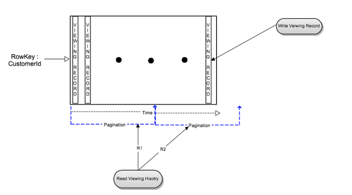
Write Flow
One viewing record was inserted as a new column when a member started playing a title. That viewing record was updated after member paused or stopped the title. This single column write was fast and efficient.
Read Flows
Whole row read to retrieve all viewing records for one member: The read was efficient when the number of records per member was small. As a member watched more titles, the number of viewing records increased. Reading rows with a large number of columns put additional stress on Cassandra that negatively impacted read latencies.
Time range query to read a time slice of a member’s data: This resulted in the same inconsistent performance as above depending on the number of viewing records within the specified time range.
Whole row read via pagination for large viewing history: This was better for Cassandra as it wasn’t waiting for all the data to be ready before sending it back. This also avoided client timeouts. However it increased overall latency to read the whole row as the number of viewing records increased.
Slowdown Reasons
Let’s look at some of the Cassandra internals to understand why our initial simple design slowed down. As the data grew, the number of SSTables increased accordingly. Since only recent data was in memory, in many cases both the memtables and SSTables had to be read to retrieve viewing history. This had a negative impact on read latency. Similarly Compaction took more IOs and time as the data size increased. Read repair and Full column repair became slower as rows got wider.
Caching Layer
Cassandra performed very well writing viewing history data but there was a need to improve the read latencies. To optimize read latencies, at the expense of increased work during the write path, we added an in-memory sharded caching layer (EVCache) in front of Cassandra storage. The cache was a simple key value store with the key being CustomerId and value being the compressed binary representation of viewing history data. Each write to Cassandra incurred an additional cache lookup and on cache hit the new data was merged with the existing value. Viewing history reads were serviced by the cache first. On a cache miss, the entry was read from Cassandra, compressed and then inserted in the cache.
With the addition of the caching layer, this single Cassandra table storage approach worked very well for many years. Partitioning based on CustomerId scaled well in the Cassandra cluster. By 2012, the Viewing History Cassandra cluster was one of the biggest dedicated Cassandra clusters at Netflix. To scale further, the team needed to double the cluster size. This meant venturing into uncharted territory for Netflix’s usage of Cassandra. In the meanwhile, Netflix business was continuing to grow rapidly, including an increasing international member base and forthcoming ventures into original content.
Redesign: Live and Compressed Storage Approach
It became clear that a different approach was needed to scale for growth anticipated over the next 5 years. The team analyzed the data characteristics and usage patterns, and redesigned viewing history storage with two main goals in mind:
- Smaller Storage Footprint.
- Consistent Read/Write Performance as viewing per member grows.
For each member, viewing history data is divided into two sets:
- Live or Recent Viewing History (LiveVH): Small number of recent viewing records with frequent updates. The data is stored in uncompressed form as in the simple design detailed above.
- Compressed or Archival Viewing History (CompressedVH): Large number of older viewing records with rare updates. The data is compressed to reduce storage footprint. Compressed viewing history is stored in a single column per row key.
LiveVH and CompressedVH are stored in different tables and are tuned differently to achieve better performance. Since LiveVH has frequent updates and small number of viewing records, compactions are run frequently and gc_grace_seconds is small to reduce number of SSTables and data size. Read repair and full column family repair are run frequently to improve data consistency. Since updates to CompressedVH are rare, manual and infrequent full compactions are sufficient to reduce number of SSTables. Data is checked for consistency during the rare updates. This obviates the need for read repair as well as full column family repair.
Write Flow
New viewing records are written to LiveVH using the same approach as described earlier.
Read Flows
To get the benefit of the new design, the viewing history API was updated with an option to read recent or full data:
- Recent Viewing History: For most cases this results in reading from LiveVH only, which limits the data size resulting in much lower latencies.
- Full Viewing History: Implemented as parallel reads of LiveVH and CompressedVH. Due to data compression and CompressedVH having fewer columns, less data is read thereby significantly speeding up reads.
CompressedVH Update Flow
While reading viewing history records from LiveVH, if the number of records is over a configurable threshold then the recent viewing records are rolled up, compressed and stored in CompressedVH via a background task. Rolled up data is stored in a new row with row key:CustomerId. The new rollup is versioned and after being written is read to check for consistency. Only after verifying the consistency of the new version, the old version of rolled up data is deleted. For simplicity there is no locking during rollup and Cassandra takes care of resolving very rare duplicate writes (i.e., the last writer wins).
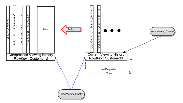
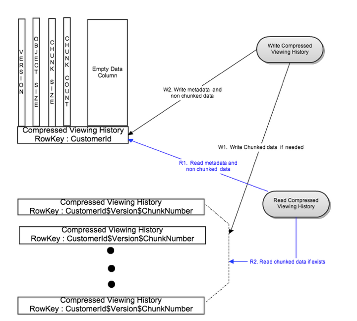
As shown in figure 2, the rolled up row in CompressedVH also stores metadata information like the latest version, object size and chunking information (more on that later). The version column stores a reference to the latest version of rolled up data so that reads for a CustomerId always return only the latest rolled up data. The rolled up data is stored in a single column to reduce compaction pressure. To minimize the frequency of rollups for members with frequent viewing pattern, just the last couple of days worth of viewing history records are kept in LiveVH after rollup and the rest are merged with the records in CompressedVH during rollup.
Auto Scaling via Chunking
For the majority of members, storing their entire viewing history in a single row of compressed data resulted in good performance during the read flows. For a small percentage of members with very large viewing history, reading CompressedVH from a single row started to slow down due to similar reasons as described in the first architecture. There was a need to have an upper bound on the read and write latencies for this rare case without negatively impacting the read and write latencies for the common case.
To solve for this, we split the rolled up compressed data into multiple chunks if the data size is greater than a configurable threshold. These chunks are stored on different Cassandra nodes. Parallel reads and writes of these chunks results in having an upper bound on the read and write latencies even for very large viewing data.
Write Flow
As figure 3 indicates, rolled up compressed data is split into multiple chunks based on a configurable chunk size. All chunks are written in parallel to different rows with row key:CustomerId$Version$ChunkNumber. Metadata is written to its own row with row key:CustomerId after successful write of the chunked data. This bounds the write latency to two writes for rollups of very large viewing data. In this case the metadata row has an empty data column to enable fast read of metadata.
To make the common case (compressed viewing data is smaller than the configurable threshold) fast, metadata is combined with the viewing data in the same row to eliminate metadata lookup overhead as shown in figure 2.
Read Flow
The metadata row is first read using CustomerId as the key. For the common case, the chunk count is 1 and the metadata row also has the most recent version of rolled up compressed viewing data. For the rare case, there are multiple chunks of compressed viewing data. Using the metadata information like version and chunk count, different row keys for the chunks are generated and all chunks are read in parallel. This bounds the read latency to two reads.
Caching Layer Changes
The in-memory caching layer was enhanced to support chunking for large entries. For members with large viewing history, it was not possible to fit the entire compressed viewing history in a single EVCache entry. So similar to the CompressedVH model, each large viewing history cache entry is broken into multiple chunks and the metadata is stored along with the first chunk.
Results
By leveraging parallelism, compression, and an improved data model, the team was able to meet all of the goals:
- Smaller Storage Footprint via compression.
- Consistent Read/Write Performance via chunking and parallel reads/writes. Latency bound to one read and one write for common cases and latency bound to two reads and two writes for rare cases.
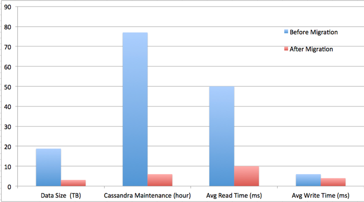
The team achieved ~6X reduction in data size, ~13X reduction in system time spent on Cassandra maintenance, ~5X reduction in average read latency and ~1.5X reduction in average write latency. More importantly, it gave the team a scalable architecture and headroom to accommodate rapid growth of Netflix viewing data.
In the next part of this blog post series, we will explore the latest scalability challenges motivating the next iteration of viewing history storage architecture. If you are interested in solving similar problems, join us.