Illustration Image

Cassandra.Link

The best knowledge base on Apache Cassandra®

Helping platform leaders, architects, engineers, and operators build scalable real time data platforms.

7/5/2017

Reading time:87 mins

Planet Cassandra

by John Doe

Sorry about missing last week, but my birthday won out overworking: Ouch! @john_overholt:My actual life is now a science exhibit about the primitiveconditions of the past.If you like this sortof Stuff then please supportme onPatreon.1PB: SSD in 1U chassis; 90%: savingsusing EC2 Spot for containers; 16:forms of inertia; $2.1B: Alibaba’s profit; 22.6B: app downloads in Q2; 25%: Google generated internet traffic; 20by 20 micrometers: quantum random number generators;16: lectures on Convolutional Neural Networks for VisualRecognition; 25,000: digitizedgramophone records; 280%: increase in IoTattacks; 6.5%:world's GDP goes to subsidizing fossil fuel; 832TB: ZFS on Linux;  $250,000:weekly take from breaking slot machines; 30: galatic message exchanges using artificial megastructuresin 100,000 years; Quotable Quotes:@chris__martin:ALIENS: we bring you a gift of reliable computing technol--HUMANS: oh no we have that already but JS is easier to hirefor@rakyll: "Youwoman, you like intern." I interned on F-16's flight computer. Evenmy internship was 100x more legit than any job you will have.@CodeWisdom:"Debugging is like being the detective in a crime movie where youare also the murderer." - Filipe FortesWilliam Gibson: what I find far more ominous is how seldom,today, we see the phrase “the 22nd century.” Almost never. Comparethis with the frequency with which the 21st century was evoked inpopular culture during, say, the 1920s.Arador: Amazon EC2, Microsoft Azure and Google Gloud Platformare all seriously screwing their customers over when it comes tobandwidth charges. Every one of the big three has massivebuying power yet between them their average bandwidth price is 3.4xhigher than colocation facilities.@mattklein123:Good thread: my view: 1) most infra startups will fail. It's anawful business to be in (sorry all, much ❤️).Jean-Louis Gassée: With Services, Apple enjoys thebenefits of a virtuous circle: Hardware sales create Servicesrevenue opportunities; Services makes hardware more attractive and“stickier”. Like Apple Stores, Services are part of the ecosystem.Such is the satisfying simplicity and robustness of Apple’sbusiness model.cardine: Theprice difference between Hetzner and AWS is large enough that itcould pay for 4x as much computational power (as much redundancy asyou'd ever need), three full time system admins (not that you'dever need them), and our office lease... with plenty of money leftover!BrujoBenavides: Communication is Key: Have you ever watched a movieor a soap opera and thought “If you would’ve just told her that, wewould’ve avoided 3 entire episodes, you moron!”. Happens to me allthe time. At Inaka we learned that the hard way.@f3ew:Doesn't matter how many layers of stateless services you have inthe middle, the interesting ends have state.brianwawok: Mycloud cost is less than 5% of my bussiness costs using GCE. Wouldbe foolish to move it to lower my costs 2%.@f3ew: Statelessservices are as relevant as routers. Pattern match, compute, pushto next layer.Horace Dediu~ when yououtsource you're taking knowledge out of your company, which endsup gutting it in terms of the value that is added JasonCalacanis: Google was the twelfth search engine. Facebook wasthe tenth social network. iPad was the twentieth tablet. It’s notwho gets there first. It’s who gets there first when the market’sready.puzzle: TheB4 paper states multiple times that Google runs links at almost100% saturation, versus the standard 30-40%. That's accomplishedthrough the use of SDN technology and, even before that, throughstrict application of QoS.@stu: Serverless has in many ways eclipsed the containersdiscussion for the hot buzz in the industry@mjpt777: GCis a wonderful thing but I cannot help but feel it leaves thetypical developer even less prepared for distributed resourcemanagement.joaodlf: Sparkworks and does a good job, it has many features that I can see ususe in the future too. With that said, it's yet another piece oftech that bloats our stack. I would love to reduce our tech debt:We are much more familiar with relational databases like MySQL andPostgres, but we fear they won't answer the analytics problems wehave, hence Cassandra and Spark. We use these technologies out ofnecessity, not love for them.tobyjsullivan: No,dear author. Setting up the AWS billing alarm was the smartestthing you ever did. It probably saved you tens of thousands ofdollars (or at least the headache associated with fighting Amazonover the bill). Developers make mistakes. It's part of thejob. It's not unusual or bad in any way. A bad developer is one whodenies that fact and fails to prepare for it. A great developer isone like the author.GeoffWozniak: Regardless of whether I find that stored proceduresaren't actually that evil or whether I keep using templated SQL, Ido know one thing: I won't fall into the "ORMs make it easy"trap.@BenedictEvans: Partof what distinguishes today’s big tech companies is a continualpush against complacency. They saw the last 20 years and read thebooksJohn Patrick Pullen: In the upcoming fall issue of Portermagazine, the 21-yer-old X-Men: Apocalypse star said, "I auditionedfor a project and it was between me and another girl who is a farbetter actress than I am, far better, but I had the followers, so Igot the job," according to The Telegraph. "It’s not right, but itis part of the movie industry now."Rachel Adler: Naturally, faster prints drove up demand forpaper, and soon traditional methods of paper production couldn’tkeep up. The paper machine, invented in France in 1799 at the Didotfamily’s paper mill, could make 40 times as much paper per day asthe traditional method, which involved pounding rags into pulp byhand using a mortar and pestle.pawelkomarnicki:As a person that can get the product from scratch to production andscale it, I can say I'm a full-stack developer. Can I feel mythicalnow?Risto: Beforeintegrating any payment flow make sure you understand the wholeflow and the different payment states trialing -> active ->unpaid -> cancelled. For Braintree there is a flow chart. ForStripe there is one too. Both payment providers have REST API’s somake sure to play through the payment flows before starting actualcoding.Seyi Fabode: I have 3 neighbors in close proximity who alsohave solar panels on their roofs. And a couple of other neighborswith electric cars. What says we can’t start our own mini-gridsystem between ourselves?pixl97: Muscles/limbsare only 'vastly' more efficient if you consider they have largenumbers of nano scale support systems constantly rebuilding them.Since we don't have nanobots, gears will be better for machines.Also, nature didn't naturally develop a axle.BraveNew Greek: I sympathize with the Go team’s desire to keepthe overall surface area of the language small and the complexitylow, but I have a hard time reconciling this with the existingbuilt-in generics and continued use of interface{} in the standardlibrary.@jeffhollan: Agreeto a point. But where does PaaS become “serverless”? Feel should be‘infinite’ scale of dynamic allocation of resources + microbill@kcimc: commontempos in 1M songs, 1959-2011: 120 bpm takes over in the late 80s,and bpms at multiples of 10 emerge in the mid 90sHow to Map the Circuits That Define Us: If neural circuits canteach one lesson, it is that no network is too small to yieldsurprises — or to frustrate attempts at comprehension.@orskov: InQ2, The Wall Street Journal had 1,270,000 daily digital-onlysubscribers, a 34% increase compared to last yearThrust Zone: A panel including tech billionaire Elon Musk isdiscussing the fact that technology has progressed so much that itmay soon destroy us and they have to pass microphones totalk.@damonedwards: Whenwe are all running containers in public clouds, I’m really going tomiss datacenter folks one-upping each other on hardwarespecs.@BenedictEvans: 186page telecoms report from 1994. 5 pages on ‘videophones’: nomention of internet. 10 pages saying web will lose to VR. Nothingon mobileThomas Metzinger: The superintelligence concludes thatnon-existence is in the own best interest of all futureself-conscious beings on this planet. Empirically, it knows thatnaturally evolved biological creatures are unable to realize thisfact because of their firmly anchored existence bias. Thesuperintelligence decides to act benevolently.Jeremy Eder: As with all public cloud, you can do whatever youwant…for a price.  BurstBalance is the creation of folks whowant you to get hooked on great performance (gp2 can run at 3000+IOPS), but then when you start doing something more than dev/testand run into these weird issues, you’re already hooked and you haveno choice but to pay more for a service that is actuallyusable.Katz and Fan: After all, the important thing for anyone lookingto launder money through a casino isn’t to win. It’s to exchangemillions of dollars for chips you can swap for cool, untraceablecash at the end of the night.Caitie McCaffrey: Verification in industry generally consistsof unit tests, monitoring, and canaries. While this provides someconfidence in the system's correctness, it is not sufficient. Moreexhaustive unit and integration tests should be written. Tools suchas random model checkers should be used to test a large subset ofthe state space. In addition, forcing a system to fail via faultinjection should be more widely used. Even simple tests such asrunning kill −9 on a primary node have found catastrophicbugs.Zupa:FPGAs give you most of the benefits of special-purpose processors,for a fraction of the cost. They are about 10x slower, but thatmeans an FPGA based bitcoin miner is still 100k times faster than aprocessor based onemenge101work: I'm not sure if the implication is that our CPUswill have gate arrays on chip with the generic CPU, that is aninteresting idea. But if they are not on chip, the gate array willnever be doing anything in a few clock cycles. It'll be more akinto going out to memory, the latency between a real memory load andan L1 or L2 cache hit is huge. (reference)Not to say that being able to do complex work on dedicatedhardware won't still be fast, but the difference between on-die andoff-die is a huge difference in how big of a change this couldbe.Animats: Thisarticle [WhyMany Smart Contract Use Cases Are Simply Impossible] outlinesthe basic problem. If you want smart contracts that do anything offchain, there have to be connections to trusted services thatprovide information and take actions. If you have trusted servicesavailable, you may not need a blockchain.The article points outthat you can't construct an ordinary loan on chain, because youhave no way to enforce paying it back short of tying up the loanedfunds tor the duration of the loan. Useful credit fundamentallyrequires some way of making debtors pay up later. It's possible toconstruct various speculative financial products entirely on chain,and that's been done, but it's mostly useful for gambling, broadlydefined.curun1r: Yourcharacterization of startup cloud costs is laughably outdated. Withcredits for startups and the ability to go serverless, I've knownstartups that didn't pay a dime for hosting their entire first yeardespite reaching the threshold of hundreds of customers and over$1m ARR. One of my friends actually started doing some ML stuff onAWS because he wanted to use his remaining credits before theyexpired and his production and staging workloads weren't going toget him there. I'd say it makes no sense to buy your 32gb,16-core single point of fail, waste $40/mo and half a day settingit up and then have to keep it running yourself when you can easilyspin up an API in API Gateway/Lambda that dumps data intodynamo/simpledb and front it with a static site in S3. That setupscales well enough to be mentioned on HN without getting hugged todeath and is kept running by someone else. And if it is, literally,free for the first year, how is that not a no brainer?Neil Irwin: In this way of thinking about productivity,inventors and business innovators are always cooking up better waysto do things, but it takes a labor shortage and high wages to coaxfirms to deploy the investment it takes to actually put thoseinnovations into widespread use. In other words, instead ofworrying so much about robots taking away jobs, maybe we shouldworry more about wages being too low for the robots to even get achance.Don't miss all that the Internet has to say on Scalability,click below and become eventually consistent with all scalabilityknowledge (which means this post has many more items to read soplease keep on reading)... 1. Hello, World!Hi, I’m Paul Brebner and this is a “Hello, World!” blog tointroduce myself and test everything out. I’m very excited to havestarted at Instaclustr last week as a Technology Evangelist.  One of the cool things to happen in my first week was thatInstaclustr celebrated a significant milestone when it exceeded 1Petabyte (1PB) of data under management.  Is this a lot ofdata? Well, yes! A Petabyte is 10^15 bytes, 1 Quadrillion bytes(which sounds more impressive!), or 1,000,000,000,000,000bytes.Also, I’m a Petabyte Person. Apart from my initials beingPB, the human brain was recently estimated to have 1PB of storagecapacity, not bad for a 1.4kg meat computer! So inthis post, I’m going to introduce myself and some of what I’velearned about Instaclustr by exploring what that Petabytemeans.Folklore has it that the 1st “Hello, World!” program waswritten in BCPL (the programming language that led to C), which Iused to program a 6809 microprocessor I built in the early 1980’s.In those days the only persistent storage I had were 8-inch floppydisks. Each disk could hold 1MB of data, so you’d need 10^9(1,000,000,000) 8-inch floppy disks to hold 1PB of data. That’s a LOT of disks, and would weigh a whopping 31,000tonnes, as much as the German WWII Pocket Battleship the AdmiralGraf Spee.Source: Wikipedia1PB of data is also a lot in terms of my experience. I worked in R&D for CSIRO and UCL in the areas ofmiddleware, distributed systems, grid computing, and sensornetworks etc between 1996-2007. During 2003 I was the softwarearchitect for a CSIRO Grid cluster computing project withBig Astronomy Data – all 2TB of it. 1PB is500,000 times more data than that.What do Instaclustr and the Large Hadron Collider have incommon?Source: cms.cernApart from the similarity of the Instaclustr Logo and theaerial shot of the LHC? (The circular pattern)Source: SequimScienceThe LHC “Data Centre processesabout one petabyte of data every day“.  Moreastonishing is that the LHC has a huge number of detectors which spit out data atthe astonishing rate of 1PB/s – most of which they don’t (andcan’t) store.2. Not just Data SizeBut there’s more to data than just the dimension of size.There are large amounts of “dead” data lying around on archivalstorage media which is more or less useless. But live dynamic datais extremely useful and is of enormous business value. So apartfrom being able to store 1PB of data (and more), you need to beable to: write data fast enough, keep track of what data you have,find the data and use it, have 24×7 availability, and havesufficient processing and storage capacity on-demand to do usefulthings as fast as possible (scalability and elasticity).  Howis this possible? Instaclustr!The Instaclustr value proposition is:“Reliability at scale.”Instaclustr solves the problem of “reliability at scale”via a combination of Scalable Open Source Big Data technologies,Public Cloud hosting, and Instaclustr’s own Managed Servicestechnologies (including cloud provisioning, cluster monitoring andmanagement, automated repairs and backups, performanceoptimization, scaling and elasticity).How does this enable reliability at Petabyte data scale?Here’s just one example. If you have 1PB+ of data on multiple SSDsin your own data centre an obvious problem would bedata durability.  1PB is a lot ofdata, and SSDs are NOT 100% error free (the main problem is“quantum tunneling” which “drills holes” in SSDs and imposes amaximum number of writes).  Thesepeople did the experiment to see how many writesit took before different SSDs died, and the answer is in some casesit’s less than 1PB. So, SSDs will fail and you will lose data –unless you have taken adequate precautions and continue to do so.The whole system must be designed and operated assuming failure isnormal.The Cassandra NoSQL database itself is designed for highdurability by replicating data on as many different nodes as youspecify (it’s basically a shared-nothing P2P distributed system). Instaclustr enhances this durability by providing automaticincremental backups (to S3 on AWS), multiple region deployments forAWS, automated repairs, and 24×7 monitoring andmanagement.3. The Data Network Effect1PB of data under management by Instaclustr is anoteworthy milestone, but that’s not the end of the story. Theamount of data will GROW! The Network effect is what happenswhen the value of a product or service increasessubstantially with the number of other people using it. The classicexample is the telephone system.  A single telephone isuseless, but 100 telephones connected together (even manually by anoperator!) is really useful, and so the network grows rapidly. DataNetwork effects are related to the amount andinterconnectedness of data in a system.  For Instaclustr customers the Data Network effect islikely to be felt in two significant ways.  Firstly, theamount of data customers have in their Cassandra cluster willincrease – as it increases over time the value will increasesignificantly; also velocity: the growth of data, services, sensorsand applications in the related ecosystems – e.g in the AWSecosystem – will accelerate.  Secondly, the continued growthin clusters and data under management provides considerable moreexperience, learned knowledge and capabilities for managingyour data and clusters.Here’s a prediction. I’ve only got 3 data points to go on.When Instaclustr started (in 2014) it was managing 0PB of data. Atthe end of 2016 this had increased to 0.5PB, and in July 2017 wereached 1PB. Assuming the amount of data continues to double at thesame rate in the future, then the total data under management byInstaclustr may increase massively over the next 3 years(Graph of Months vs PB of data).4. What next?I started as Technology Evangelist at Instaclustr (lastweek). My background for the last 10 years has been a seniorresearch scientist in NICTA (National ICT Australia, now mergedwith CSIRO as Data61), and for the last few years at CTO/consultantwith a NICTA start-up specializing in performance engineering (viaPerformance Data Analytics and Modelling). I’ve invented someperformance analytics techniques, commercialized them in a tool,and applied them to client problems, often in the context of BigData Analytics problems. The tool we developed actually usedCassandra (but in a rather odd way, we needed to store very largevolumes of performance data for later analysis from a simulationengine, hours of data could be simulated and needed to be persistedin a few seconds and Cassandra was ideal for that use case). I’malso an AWS Associate Solution Architect. Before all this, I was aComputer Scientist, Machine Learning researcher, Software Engineer,Software Architect, UNIX systems programmer, etc.  Some ofthis may come in useful for getting up to speed with Cassandraetc.Over the next few months, the plan is for me to understandthe Instaclustr technologies from “end user” and developerperspectives, develop and try out some sample applications, andblog about them. I’m going to start with the internal Instaclustruse case for Cassandra, which is the heart of the performance datamonitoring tool (Instametrics). Currently there’s lots of performance data stored inCassandra, but only a limited amount of analysis and predictionbeing done (just aggregation). It should be feasible and aninteresting learning exercise to do some performance analytics onthe Cassandra data performance data to predict interesting eventsin advance and take remedial action.I’m planning to start out with some basic use cases andprogramming examples for Cassandra (e.g. how do you connect toCassandra, how do you find out what’s in it, how do get data out ofit, how do you do simple queries such as finding “outliers”, how doyou more complex Data Analytics (e.g. regression analysis, ML,etc), etc. I’ll probably start out very simple. e.g. Cassandra& Java on my laptop, having a look at some sample Cassandradata, try some simple Data analytics, then move to more complexexamples as the need arises. E.g. Cassandra on Instaclustr, Java onAWS, Spark + MLLib, etc. I expect to make some mistakes and revisethings as I go. Most of all I hope to make itinteresting.Watch this space The post Paul Brebner (the Petabyte Person) joins Instaclustr (the PetabyteCompany) appeared first on Instaclustr. A handy feature was silently added to Apache Cassandra’s nodetool just over a year ago. Thefeature added was the -j(jobs) option. This little gem controls the number of compactionthreads to use when running either a scrub, cleanup, or upgradesstables. The option was added tonodetool via CASSANDRA-11179to version 3.5. It has been back ported to Apache Cassandraversions 2.1.14, 2.2.6, and 3.5.If unspecified, nodetoolwill use 2 compaction threads. When this value is set to 0 allavailable compaction threads are used to perform the operation.Note that the total number of available compaction threads iscontrolled by the concurrent_compactors property in thecassandra.yaml configuration file. Examples of how it canbe used are as follows.$ nodetool scrub -j 3$ nodetool cleanup -j 1$ nodetool upgradesstables -j 1 The option is most useful in situations where disk space isscarce and a limited number of threads for the operation need to beused to avoid disk exhaustion. Introduction I’ve wanted to create a system which inits core uses event sourcing for quite a while - actually sinceI’ve read Martin Kleppmann’s MakingSense of Stream Processing. The book isreally amazing, Martin tends to explain all concepts from basicbuilding blocks and in a really simple and understandable way. Irecommend it to everyone. The idea is to have a running Cassandracluster and to evolve a system with no downtime in such a way thatKafka is the Source of Truth with immutable facts. Every othersystem (in this case Cassandra cluster) should use these facts andaggregate / transform them for its purpose. Also, since all factsare in Kafka, it should be easy to drop the whole database, index,cache or any other data system and recreate it from scratchagain. Thefollowing diagrams should illustrate the systemevolution. Starting systemarchitecture   Target systemarchitecture   When observing the diagrams, it seems likea pretty straightforward and trivial thing to do, but there’s moreto it, especially when you want to do it with nodowntime. Evolutionbreakdown Itried to break down the evolution process to a few conceptual stepsand this is what I came up with: Have a mechanism to push each Cassandrachange to Kafka with timestampStart collecting each Cassandra change totemporary Kafka topic I need to start collecting before asnapshot is taken, otherwise there will be a time window in whichincoming changes would be lost, and it also needs to go totemporary topic since there is data in the database which should befirst in an ordered sequence of events Take the existing databasesnapshot This one ispretty straightforward Start reading data from the snapshot intothe right Kafka topic Since the data from the snapshot wascreated first, it should be placed first intoKafka After the snapshot is read, redirect thedata from the temporary Kafka topic to the right Kafka topic, butmind the timestamp when the snapshot is taken This step is essential to be donecorrectly, and could be considered as the hardest part. Sincechange event collecting started before the snapshot, there is apossibility that some events also exist in the snapshot as welland, to avoid inconsistencies, each event should be idempotent andI should try to be as precise as possible when comparing the eventtimestamp with the snapshot timestamp Create a new Cassandracluster/keyspace/table and Kafka stream to read from Kafka andinsert into this new Cassandracluster/keyspace/table As a result, the new cassandra clustershould be practically a copy/clone of the existingone Waitfor the temporary Kafka topic to deplete If I change the application to read fromthe new cassandra right away, and Kafka temporary topic stilldoesn’t catch up with system, there will be significant read delays(performance penalties) in the system. To make sure everything isin order, I think monitoring of time to propagate the change to thenew Cassandra cluster will help and if the number is decent (a fewmilliseconds), I can proceed to the nextstep Change the application to read from the newcassandra instead of old and still write to oldSince everything is done within theno downtime context, the application is actually several instancesof application on different nodes, and they won’t be changedsimultaneously, that would cause the downtime. I’d need to changeone at a time, while others are still having the old softwareversion. For this reason, the application still needs to write tothe old cassandra, since other application nodes are still readingfrom the old cassandra. When each application instance is updated,change the application to write directly to Kafka righttopic Now each node,one by one, can be updated with new application version which willwrite directly to Kafka. In parallel, old nodes will write to theold Cassandra which will propagate to Kafka topic, and new nodeswill write directly to the Kafka topic. When the change iscomplete, all nodes are writing directly to the Kafka topic and weare good to go. Clean up At this point, the system writes to theright Kafka topic, the stream is reading from it and making insertsinto the new Cassandra. The old Cassandra and Kafka temporary topicare no longer necessary so it should be safe for me to removethem. Well, that’s the plan, so we’ll seewhether it is doable or not. There are a few motivating factors whyI’ve chosen to evolve an existing system instead of building onethe way I want from scratch. It is more challenging, hence morefun The need forevolving existing systems is the everyday job of softwaredevelopers; you don’t get a chance to build a system for a startingset of requirements with guarantee that nothing in it will everchange (except for a college project,perhaps) When asystem needs to change, you can choose two ways, to build a new onefrom scratch and when ready replace the old or to evolve theexisting. I’ve done the former a few times in my life, and it mightseem as fun at the beginning, but it takes awfully long, with a lotof bug fixing, often ends up as a catastrophe and is alwaysexpensive Evolving asystem takes small changes with more control, instead of placing atotally new system instead of the old.I’m a fan of Martin Fowler’s blog,EvolutionaryDatabase Design fitsparticularly nicely in this topic Since writing about thisin a single post would render quite a huge post, I’ve decided tosplit it into a few, I’m still not sure how many, but I’ll startand see where it takes me. Bear with me.Data modelI’ll start with data model.Actually, it is just one simple table, but it should be enough todemonstrate the idea. The following CQL code describes thetable. CREATETABLE IF NOT EXISTS movies_by_genre (title text,genre text,year int,ratingfloat,duration int,director text,country text,PRIMARY KEY ((genre, year), rating,duration)) WITH CLUSTERING ORDER BY (rating DESC,duration ASC) The usecase for this table might not be that common, since the table isactually designed to have a complex primary key with at least twocolumns as a partition key and at least two clustering columns. Thereason for that is it will leverage examples, since handling of acomplex primary key might be needed for someone readingthis. Inorder to satisfy the first item from the Evolution breakdown, Ineed a way to push each Cassandra change to Kafka with a timestamp.There are a few ways to do it: Cassandra Triggers, Cassandra CDC,Cassandra Custom Secondary Index and possibly some other ways, butI’ll investigate only the three mentioned.CassandraTriggers Forthis approach I’ll use two Cassandra 3.11.0 nodes, two Kafka0.10.1.1 nodes and one Zookeeper 3.4.6. Every node will run in aseparate Docker container. I decided to use Docker since it keepsmy machine clean and it is easy to recreateinfrastructure. To create a trigger in Cassandra, ITriggerinterface needs to be implemented. The interface itself is prettysimple: publicinterface ITrigger {publicCollection<Mutation> augment(Partition update);} And that’s allthere is to it. The interface has been changed since Cassandra 3.0.Earlier versions of Cassandra used the followinginterface: public interface ITrigger {public Collection<Mutation> augment(ByteBufferpartitionKey, ColumnFamily update);} Before I dive into implementation, let’sdiscuss the interface a bit more. There are several importantpoints regarding the implementation that need to be honored andthose points are explained on the interface’sjavadoc: Implementation of this interface should onlyhave a constructor without parametersITrigger implementation canbe instantiated multiple times during the server life time.(Depends on the number of times the trigger folder isupdated.) ITriggerimplementation should be stateless (avoid dependency on instancevariables). Besides that, augment method is calledexactly once per update and Partition object containsall relevant information about the update. You might notice thatreturn type is not void but rather a collectionof mutations. This way trigger can be implemented to perform someadditional changes when certain criteria are met. But since I justwant to propagate data to Kafka, I’ll just read the updateinformation, send it to Kafka and return empty mutation collection.In order not to pollute this article with a huge amount of code,I’ve created maven project which creates a JAR file, and theproject can be found here.I’ll try to explain the code in theproject. Firstly, there is a FILE_PATH constant, whichpoints to /etc/cassandra/triggers/KafkaTrigger.ymland this is where YAML configuration for trigger class needs to be.It should contain configuration options for Kafka brokers and fortopic name. The file is pretty simple, since the whole filecontains just the following two lines:bootstrap.servers:cluster_kafka_1:9092,cluster_kafka_2:9092 topic.name:trigger-topic I’ll cometo that later when we build our docker images. Next, there is aconstructor which initializes the Kafka producer and ThreadPoolExecutor. I couldhave done it without ThreadPoolExecutor, but thereason for it is that the trigger augment call is onCassandra’s write path and in that way it impacts Cassandra’s writeperformances. To minimize that, I’ve moved trigger execution tobackground thread. This is doable in this case, since I am notmaking any mutations, I can just start the execution in anotherthread and return an empty list of mutations immediately. In casewhen the trigger needs to make a mutation based on partitionchanges, that would need to happen in the samethread. Reading data from partition update inaugment method is really a mess. Cassandra API is not thatintuitive and I went through a real struggle to read all thenecessary information. There are a few different ways to update apartition in Cassandra, and these are ones I’vecovered: InsertUpdateDelete of directorcolumn Delete oftitle column Deleteof both director and title columnsDelete of rowDelete range of rows for last clusteringcolumn (duration between some values)Delete all rows for specific ratingclustering columnDelete range of rows for first clusteringcolumn (rating between some values)Delete wholepartition A simplified algorithm wouldbe: if(isPartitionDeleted(partition)) {handle partitiondelete;} else {if(isRowUpdated(partition)) {if(isRowDeleted(partition)) {handle row delete;} else {if (isCellDeleted(partition)) {handle cell delete;} else {handleupsert;}}} else if(isRangeDelete(partition)) {handle range delete;}} Ineach case, JSON is generated and sent to Kafka. Each messagecontains enough information to recreate Cassandra CQL query fromit. Besidesthat, there are a few helper methods for reading the YAMLconfiguration and that is all. In order to test everything, I’ve chosenDocker, as stated earlier. I’m using Cassandradocker image with 3.11.0 tag. But since the JAR file and KafkaTrigger.yml need to becopied into the docker container, there are twooptions: Use Cassandra 3.11.0 image and docker cpcommand to copy the files into thecontainer Create anew Docker image with files already in it and use thatimage The first option is not an optionactually, it is not in the spirit of Docker to do such thing so Iwill go with the second option. Create a cluster directory somewhere and acassandra directory within it mkdir -p cluster/cassandra cluster directory will beneeded for later, now just create KafkaTrigger.yml incassandra dir with the content I provided earlier. Also, the builtJAR file (cassandra-trigger-0.0.1-SNAPSHOT.jar)needs to be copied here. To build all that into Docker, I created aDockerfile with the following content:FROM cassandra:3.11.0COPYKafkaTrigger.yml /etc/cassandra/triggers/KafkaTrigger.ymlCOPY cassandra-trigger-0.0.1-SNAPSHOT.jar/etc/cassandra/triggers/trigger.jarCMD ["cassandra","-f"] In console, justposition yourself in the cassandra directory andrun: dockerbuild -t trigger-cassandra . That will create a docker image with nametrigger-cassandra.All that is left is to create aDocker compose file, join all together and test it. The Dockercompose file should be placed in the  cluster directory. Thereason for that is because Docker compose has a naming conventionfor containers it creates, it is <present_directory_name>_<service_name>_<order_num>.And I already specified the Kafka domain names in KafkaTrigger.yml as cluster_kafka_1 and cluster_kafka_2, in case theDocker compose is run from another location, container naming wouldchange and KafkaTrigger.yml would needto be updated. My Docker compose file is located inthe cluster directory, it’s named cluster.yml and it lookslike this: version: '3.3'services:zookeeper:image:wurstmeister/zookeeper:3.4.6ports:-"2181:2181"kafka:image:wurstmeister/kafka:0.10.1.1ports:-9092environment:HOSTNAME_COMMAND:"ifconfig | awk '/Bcast:.+/{print $$2}' | awk -F\":\" '{print$$2}'"KAFKA_ADVERTISED_PORT: 9092KAFKA_ZOOKEEPER_CONNECT: zookeeper:2181cassandra-seed:image: trigger-cassandraports:- 7199- 9042environment:CASSANDRA_CLUSTER_NAME: test-clustercassandra:image: trigger-cassandraports:- 7199- 9042environment:CASSANDRA_CLUSTER_NAME: test-clusterCASSANDRA_SEEDS: cassandra-seed The cluster contains the definition forZookeeper, Kafka and Cassandra with the exception that there aretwo Cassandra services. The reason for that is that one can bestandalone, but all others need a seed list. cassandra-seed will serve asseed, and cassandra as scalableservice. That way, I can start multiple instances of cassandra.However, to start multiple instances, it takes time, and it is notrecommended to have multiple Cassandra nodes in joining state. So,scale should be done one node at a time. That does not apply toKafka nodes. With the following command, I’ve got a running clusterready for use: docker-compose -f cluster.yml up -d --scalekafka=2 After that, Iconnected to the Cassandra cluster with cqlsh andcreated the keyspace and table. To add a trigger to the table, you need toexecute the following command: CREATE TRIGGER kafka_trigger ONmovies_by_genre USING'io.smartcat.cassandra.trigger.KafkaTrigger'; In case you get the followingerror: ConfigurationException: Trigger class'io.smartcat.cassandra.trigger.KafkaTrigger' doesn'texist There are severalthings that can be wrong. The JAR file might not be loaded withinthe Cassandra node; that should happen automatically, but if itdoesn’t you can try to load it with: nodetool reloadTriggers If the problem persists, it might be thatthe configuration file is not at a proper location, but that canonly happen if you are using a different infrastructure setup andyou forgot to copy KafkaTrigger.yml to theproper location. Cassandra will show the same error even if classis found but there is some problem instantiating it or casting itto theITrigger interface. Also, make sure that you implemented theITriggerinterface from the right Cassandra version (versions of cassandrain the JAR file and of the cassandra node shouldmatch). Ifthere are no errors, the trigger is created properly. This can bechecked by executing the following CQLcommands: USEsystem_schema;SELECT * FROM triggers;ResultsI used kafka-console-consumer to seeif messages end up in Kafka, but any other option is good enough.Here are a few things I tried and the results it gaveme. For most cases, not all of these mutationsare used, usually it’s just insert, update and one kind of delete.Here I intentionally tried several ways since it might come inhandy to someone. In case you have a simpler table use case, youmight be able to simplify the trigger code aswell. What isalso worth noting is that triggers execute only on a coordinatornode; they have nothing to do with data ownership nor replicationand the JAR file needs to be on every node that can become acoordinator. Going a stepfurther Thisis OK for testing purposes, but for this experiment to have anyvalue, I will simulate the mutations to the cassandra cluster atsome rate. This can be accomplished in several ways, writing acustom small application, using cassandra stress or using someother tool. Here at SmartCat, we have developed a tool for suchpurpose. That is the easiest way for me to create load on aCassandra cluster. The tool is called Berserker,you can give it a try. To start with Berserker, I’ve downloadedthe latest version (0.0.7 is the latest at the moment of writing)from here.And I’ve created a configuration file namedconfiguration.yml. load-generator-configurationsection is used to specify all other configurations. There, forevery type of the configuration, name is specified in order for theBerserker to know which configuration parser to use in concretesections. After that, a section for each configuration with parserspecific options and format is found. There are following sectionsavailable: data-source-configurationwhere data source which will generate data for worker isspecified rate-generator-configurationwhere should be specified how rate generator will be created and itwill generate rate. This rate is rate at which worker willexecute worker-configuration,configuration for workermetrics-reporter-configuration,configuration for metrics reporting, currently only JMX and consolereporting is supported In this case, the data-source-configurationsection is actually a Ranger configuration format and can be foundhere.An important part for this articleis the connection-points propertywithin worker-configration. Thiswill probably be different every time Docker compose creates acluster. To see your connection points run:docker ps It should give you a similaroutput: There you can find port mapping forcluster_cassandra-seed_1 andcluster_cassandra_1containers and use it, in this case it is: 0.0.0.0:32779 and 0.0.0.0:32781.Now that everything is settled, justrun: java -jarberserker-runner-0.0.7.jar -c configuration.yml Berserker starts spamming the Cassandracluster and in my terminal where kafka-console-consumer isrunning, I can see messages appearing, it seems everything is asexpected, at least for now. EndThat’s all, next time I’ll talkabout Cassandra CDC and maybe custom secondary index. Hopefully, ina few blog posts, I’ll have the whole idea tested andrunning. One of the common griefs Scala developers express when using theDataStax Java driver is the overhead incurred in almost every reador write operation, if the data to be stored or retrieved needsconversion from Java to Scala or vice versa.This could be avoided by using "native" Scala codecs. This hasbeen occasionally solicited from the Java driver team, but suchcodecs unfortunately do not exist, at least not officially.Thankfully, the TypeCodec API in the Java driver can be easily extended. Forexample, several convenience Java codecs are available in the driver's extras package.In this post, we are going to piggyback on the existing extracodecs and show how developers can create their own codecs –directly in Scala.Note: all the examples in this post are available inthisGithub repository.Dealing with NullabilityIt can be tricky to deal with CQL types in Scala because CQLtypes are all nullable, whereas most typical representations of CQLscalar types in Scala resort to value classes, and these arenon-nullable.As an example, let's see how the Java driver deserializes, say,CQL ints.The default codec for CQL ints converts such values tojava.lang.Integer instances. From a Scala perspective,this has two disadvantages: first, one needs to convert fromjava.lang.Integer to Int, and second,Integer instances are nullable, while ScalaInts aren't.Granted, the DataStax Java driver's Row interfacehas a pair of methods named getInt that deserialize CQL ints intoJava ints, converting null values intozeroes.But for the sake of this demonstration, let's assume that thesemethods did not exist, and all CQL ints were beingconverted into java.lang.Integer. Therefore,developers would yearn to have a codec that could deserialize CQLints into Scala Ints while at the sametime addressing the nullability issue.Let this be the perfect excuse for us to introduceIntCodec, our first Scala codec:import java.nio.ByteBufferimport com.datastax.driver.core.exceptions.InvalidTypeExceptionimport com.datastax.driver.core.{DataType, ProtocolVersion, TypeCodec}import com.google.common.reflect.TypeTokenobject IntCodec extends TypeCodec[Int](DataType.cint(), TypeToken.of(classOf[Int]).wrap()) { override def serialize(value: Int, protocolVersion: ProtocolVersion): ByteBuffer = ByteBuffer.allocate(4).putInt(0, value) override def deserialize(bytes: ByteBuffer, protocolVersion: ProtocolVersion): Int = { if (bytes == null || bytes.remaining == 0) return 0 if (bytes.remaining != 4) throw new InvalidTypeException("Invalid 32-bits integer value, expecting 4 bytes but got " + bytes.remaining) bytes.getInt(bytes.position) } override def format(value: Int): String = value.toString override def parse(value: String): Int = { try { if (value == null || value.isEmpty || value.equalsIgnoreCase("NULL")) 0 else value.toInt } catch { case e: NumberFormatException => throw new InvalidTypeException( s"""Cannot parse 32-bits integer value from "$value"""", e) } }}All we did so far is extend TypeCodec[Int] byfilling in the superclass constructor arguments (more about thatlater) and implementing the required methods in a very similar waycompared to the driver's built-in codec.Granted, this isn't rocket science, but it will get moreinteresting later. The good news is, this template is reproducibleenough to make it easy for readers to figure out how to createsimilar codecs for every AnyVal that is mappable to aCQL type (Boolean, Long,Float, Double, etc... let yourimagination run wild or just go for the ready-made solution).(Tip: because of the automatic boxing/unboxing that occurs underthe hood, don't use this codec to deserialize simple CQLints, and prefer instead the driver's built-in one,which will avoid this overhead; but you can useIntCodec to compose more complex codecs, as we willsee below – the more complex the CQL type, the more negligible theoverhead becomes.)Let's see how this piece of code solves our initial problems: asfor the burden of converting between Scala and Java,Int values are now written directly withByteBuffer.putInt, and read directly fromByteBuffer.getInt; as for the nullability of CQLints, the issue is addressed just as the driver does:nulls are converted to zeroes.Converting nulls into zeroes might not besatisfying for everyone, but how to improve the situation? Thegeneral Scala solution for dealing with nullable integers is to mapthem to Option[Int]. DataStax Spark Connector forApache Cassandra®'s CassandraRow class has exactly one suchmethod:def getIntOption(index: Int): Option[Int] = ...Under the hood, it reads a java.lang.Integer fromthe Java driver's Row class, and converts the value toeither None if it's null, or toSome(value), if it isn't.Let's try to achieve the same behavior, but using the compositepattern: we first need a codec that converts from any CQLvalue into a Scala Option. There is no such built-incodec in the Java driver, but now that we are codec experts, let'sroll our own OptionCodec:class OptionCodec[T]( cqlType: DataType, javaType: TypeToken[Option[T]], innerCodec: TypeCodec[T]) extends TypeCodec[Option[T]](cqlType, javaType) with VersionAgnostic[Option[T]] { def this(innerCodec: TypeCodec[T]) { this(innerCodec.getCqlType, TypeTokens.optionOf(innerCodec.getJavaType), innerCodec) } override def serialize(value: Option[T], protocolVersion: ProtocolVersion): ByteBuffer = if (value.isEmpty) OptionCodec.empty.duplicate else innerCodec.serialize(value.get, protocolVersion) override def deserialize(bytes: ByteBuffer, protocolVersion: ProtocolVersion): Option[T] = if (bytes == null || bytes.remaining() == 0) None else Option(innerCodec.deserialize(bytes, protocolVersion)) override def format(value: Option[T]): String = if (value.isEmpty) "NULL" else innerCodec.format(value.get) override def parse(value: String): Option[T] = if (value == null || value.isEmpty || value.equalsIgnoreCase("NULL")) None else Option(innerCodec.parse(value))}object OptionCodec { private val empty = ByteBuffer.allocate(0) def apply[T](innerCodec: TypeCodec[T]): OptionCodec[T] = new OptionCodec[T](innerCodec) import scala.reflect.runtime.universe._ def apply[T](implicit innerTag: TypeTag[T]): OptionCodec[T] = { val innerCodec = TypeConversions.toCodec(innerTag.tpe).asInstanceOf[TypeCodec[T]] apply(innerCodec) }}And voilà! As you can see, the class body is very simple (itscompanion object is not very exciting at this point either, but wewill see later how it could do more than just mirror the classconstructor). Its main purpose when deserializing/parsing is todetect CQL nulls and return None rightaway, without even having to interrogate the inner codec,and when serializing/formatting, intercept None sothat it can be immediately converted back to an emptyByteBuffer (the native protocol's representation ofnull).We can now combine our two codecs together,IntCodec and OptionCodec, and compose aTypeCodec[Option[Int]]:import com.datastax.driver.core._val codec: TypeCodec[Option[Int]] = OptionCodec(IntCodec)assert(codec.deserialize(ByteBuffer.allocate(0), ProtocolVersion.V4).isEmpty)assert(codec.deserialize(ByteBuffer.allocate(4), ProtocolVersion.V4).isDefined)The problem with TypeTokensLet's sum up what we've got so far: aTypeCodec[Option[Int]] that is the perfect match forCQL ints. But how to use it?There is nothing really particular with this codec and it isperfectly compatible with the Java driver. You can use itexplicitly, which is probably the simplest way:import com.datastax.driver.core._val codec: TypeCodec[Option[Int]] = OptionCodec(IntCodec)val row: Row = ??? // some CQL query containing an int columnval v: Option[Int] = row.get(0, codec)But your application is certainly more complex than that, andyou would like to register your codec beforehand so that it getstransparently used afterwards:import com.datastax.driver.core._// firstval codec: TypeCodec[Option[Int]] = OptionCodec(IntCodec)cluster.getConfiguration.getCodecRegistry.register(codec)// thenval row: Row = ??? // some CQL query containing an int columnval v: Option[Int] = row.get(0, ???) // How to get a TypeToken[Option[Int]]?Well, before we can actually do that, we first need to solve oneproblem: the Row.get method comes in a few overloadedflavors, and the most flavory ones accept a TypeToken argument; let's learn how to use them inScala.The Java Driver API, for historical reasons — but also, let's behonest, due to the lack of alternatives – makes extensive usage ofGuava'sTypeToken API (if you are not familiar with the typetoken pattern you might want to stop and read about itfirst).Scala has its own interpretation of the same reflective pattern,named type tags. Both APIs pursue identical goals – toconvey compile-time type information to the runtime – throughvery different roads. Unfortunately, it's all but an easy path totravel from one to the other, simply because there is no easy bridge between java.lang.Type and Scala'sType.Hopefully, all is not lost. As a matter of fact, creating afull-fledged conversion service between both APIs is not apre-requisite: it turns out that Guava's TypeTokenworks pretty well in Scala, and most classes get resolved justfine. TypeTokens in Scala are just a bit cumbersome touse, and quite error-prone when instantiated, but that's somethingthat a helper object can facilitate.We are not going to dive any deeper in the troubled waters ofScala reflection (well, at least not until the last chapter of thistutorial). It suffices to assume that the helper object wementioned above really exists, and that it does the job of creatingTypeToken instances while at the same time sparing thedeveloper the boiler-plate code that this operation usuallyincurs.Now we can resume our example and complete our code that reads aCQL int into a Scala Option[Int], in themost transparent way:import com.datastax.driver.core._val tt = TypeTokens.optionOf(TypeTokens.int) // creates a TypeToken[Option[Int]]val row: Row = ??? // some CQL query containing an int columnval v: Option[Int] = row.get(0, tt) Dealing with CollectionsAnother common friction point between Scala and the Java driveris the handling of CQL collections.Of course, the driver has built-in support for CQL collections;but obviously, these map to typical Java collection types: CQLlist maps to java.util.List (implementedby java.util.ArrayList), CQL set tojava.util.Set (implemented byjava.util.LinkedHashSet) and CQL map tojava.util.Map (implemented byjava.util.HashMap).This leaves Scala developers with two inglorious options:Use the implicit JavaConverters object and deal with – gasp! –mutable collections in their code;Deal with custom Java-to-Scala conversion in their code, andface the consequences of conversion overhead (this is the choicemade by the already-mentioned Spark Connector for ApacheCassandra®, because it has a very rich set of convertersavailable).All of this could be avoided if CQL collection types weredirectly deserialized into Scala immutable collections.Meet SeqCodec, our third Scala codec in thistutorial:import java.nio.ByteBufferimport com.datastax.driver.core.CodecUtils.{readSize, readValue}import com.datastax.driver.core._import com.datastax.driver.core.exceptions.InvalidTypeExceptionclass SeqCodec[E](eltCodec: TypeCodec[E]) extends TypeCodec[Seq[E]]( DataType.list(eltCodec.getCqlType), TypeTokens.seqOf(eltCodec.getJavaType)) with ImplicitVersion[Seq[E]] { override def serialize(value: Seq[E], protocolVersion: ProtocolVersion): ByteBuffer = { if (value == null) return null val bbs: Seq[ByteBuffer] = for (elt <- value) yield { if (elt == null) throw new NullPointerException("List elements cannot be null") eltCodec.serialize(elt, protocolVersion) } CodecUtils.pack(bbs.toArray, value.size, protocolVersion) } override def deserialize(bytes: ByteBuffer, protocolVersion: ProtocolVersion): Seq[E] = { if (bytes == null || bytes.remaining == 0) return Seq.empty[E] val input: ByteBuffer = bytes.duplicate val size: Int = readSize(input, protocolVersion) for (_ <- 1 to size) yield eltCodec.deserialize(readValue(input, protocolVersion), protocolVersion) } override def format(value: Seq[E]): String = { if (value == null) "NULL" else '[' + value.map(e => eltCodec.format(e)).mkString(",") + ']' } override def parse(value: String): Seq[E] = { if (value == null || value.isEmpty || value.equalsIgnoreCase("NULL")) return Seq.empty[E] var idx: Int = ParseUtils.skipSpaces(value, 0) if (value.charAt(idx) != '[') throw new InvalidTypeException( s"""Cannot parse list value from "$value", at character $idx expecting '[' but got '${value.charAt(idx)}'""") idx = ParseUtils.skipSpaces(value, idx + 1) val seq = Seq.newBuilder[E] if (value.charAt(idx) == ']') return seq.result while (idx < value.length) { val n = ParseUtils.skipCQLValue(value, idx) seq += eltCodec.parse(value.substring(idx, n)) idx = n idx = ParseUtils.skipSpaces(value, idx) if (value.charAt(idx) == ']') return seq.result if (value.charAt(idx) != ',') throw new InvalidTypeException( s"""Cannot parse list value from "$value", at character $idx expecting ',' but got '${value.charAt(idx)}'""") idx = ParseUtils.skipSpaces(value, idx + 1) } throw new InvalidTypeException( s"""Malformed list value "$value", missing closing ']'""") } override def accepts(value: AnyRef): Boolean = value match { case seq: Seq[_] => if (seq.isEmpty) true else eltCodec.accepts(seq.head) case _ => false }}object SeqCodec { def apply[E](eltCodec: TypeCodec[E]): SeqCodec[E] = new SeqCodec[E](eltCodec)}(Of course, we are talking here aboutscala.collection.immutable.Seq.)The code above is still vaguely ressemblant to the equivalent Java code, and not very interesting per se;the parse method in particular is not exactly a feastfor the eyes, but there's little we can do about it.In spite of its modest body, this codec allows us to compose amore interesting TypeCodec[Seq[Option[Int]]] that canconvert a CQL list<int> directly into ascala.collection.immutable.Seq[Option[Int]]:import com.datastax.driver.core._type Seq[+A] = scala.collection.immutable.Seq[A]val codec: TypeCodec[Seq[Int]] = SeqCodec(OptionCodec(IntCodec))val l = List(Some(1), None)assert(codec.deserialize(codec.serialize(l, ProtocolVersion.V4), ProtocolVersion.V4) == l)Some remarks about this codec:This codec is just for the immutable Seq type. Itcould be generalized into an AbstractSeqCodec in orderto accept other mutable or immutable sequences. If you want to knowhow it would look, the answer is here.Ideally, TypeCodec[T] should have been madecovariant in T, the type handled by the codec (i.e.TypeCodec[+T]); unfortunately, this is not possible inJava, so TypeCodec[T] is in practice invariant inT. This is a bit frustrating for Scala implementors,as they need to choose the best upper bound for T, andstick to it for both input and output operations, just like we didabove.Similar codecs can be created to map CQL sets toSets and CQL maps to Maps; again, we leave this as an exercise to theuser (and again, it is possible to cheat).Dealing with TuplesScala tuples are an appealing target for CQL tuples.The Java driver does have a built-in codec for CQL tuples; butit translates them into TupleValue instances, which are unfortunately oflittle help for creating Scala tuples.Luckily enough, TupleCodec inherits from AbstractTupleCodec, a class that has been designedexactly with that purpose in mind: to be extended by developerswanting to map CQL tuples to more meaningful types thanTupleValue.As a matter of fact, it is extremely simple to craft a codec forTuple2by extending AbstractTupleCodec:class Tuple2Codec[T1, T2]( cqlType: TupleType, javaType: TypeToken[(T1, T2)], eltCodecs: (TypeCodec[T1], TypeCodec[T2])) extends AbstractTupleCodec[(T1, T2)](cqlType, javaType) with ImplicitVersion[(T1, T2)] { def this(eltCodec1: TypeCodec[T1], eltCodec2: TypeCodec[T2])(implicit protocolVersion: ProtocolVersion, codecRegistry: CodecRegistry) { this( TupleType.of(protocolVersion, codecRegistry, eltCodec1.getCqlType, eltCodec2.getCqlType), TypeTokens.tuple2Of(eltCodec1.getJavaType, eltCodec2.getJavaType), (eltCodec1, eltCodec2) ) } { val componentTypes = cqlType.getComponentTypes require(componentTypes.size() == 2, s"Expecting TupleType with 2 components, got ${componentTypes.size()}") require(eltCodecs._1.accepts(componentTypes.get(0)), s"Codec for component 1 does not accept component type: ${componentTypes.get(0)}") require(eltCodecs._2.accepts(componentTypes.get(1)), s"Codec for component 2 does not accept component type: ${componentTypes.get(1)}") } override protected def newInstance(): (T1, T2) = null override protected def serializeField(source: (T1, T2), index: Int, protocolVersion: ProtocolVersion): ByteBuffer = index match { case 0 => eltCodecs._1.serialize(source._1, protocolVersion) case 1 => eltCodecs._2.serialize(source._2, protocolVersion) } override protected def deserializeAndSetField(input: ByteBuffer, target: (T1, T2), index: Int, protocolVersion: ProtocolVersion): (T1, T2) = index match { case 0 => Tuple2(eltCodecs._1.deserialize(input, protocolVersion), null.asInstanceOf[T2]) case 1 => target.copy(_2 = eltCodecs._2.deserialize(input, protocolVersion)) } override protected def formatField(source: (T1, T2), index: Int): String = index match { case 0 => eltCodecs._1.format(source._1) case 1 => eltCodecs._2.format(source._2) } override protected def parseAndSetField(input: String, target: (T1, T2), index: Int): (T1, T2) = index match { case 0 => Tuple2(eltCodecs._1.parse(input), null.asInstanceOf[T2]) case 1 => target.copy(_2 = eltCodecs._2.parse(input)) }}object Tuple2Codec { def apply[T1, T2](eltCodec1: TypeCodec[T1], eltCodec2: TypeCodec[T2]): Tuple2Codec[T1, T2] = new Tuple2Codec[T1, T2](eltCodec1, eltCodec2)}A very similar codec for Tuple3can be found here. Extending this principle to Tuple4,Tuple5, etc. is straightforward and left for thereader as an exercise.Going incognito with implicitsThe careful reader noticed that Tuple2Codec'sconstructor takes two implicit arguments: CodecRegistry and ProtocolVersion. They are omnipresent in theTypeCodec API and hence, good candidates for implicitarguments – and besides, both have nice default values. To make thecode above compile, simply put in your scope something along thelines of:object Implicits { implicit val protocolVersion = ProtocolVersion.NEWEST_SUPPORTED implicit val codecRegistry = CodecRegistry.DEFAULT_INSTANCE}Speaking of implicits, let's now see how we can simplify ourcodecs by adding a pinch of those. Let's take a look at our firsttrait in this tutorial:trait VersionAgnostic[T] { this: TypeCodec[T] => def serialize(value: T)(implicit protocolVersion: ProtocolVersion, marker: ClassTag[T]): ByteBuffer = this.serialize(value, protocolVersion) def deserialize(bytes: ByteBuffer)(implicit protocolVersion: ProtocolVersion, marker: ClassTag[T]): T = this.deserialize(bytes, protocolVersion)}This trait basically creates two overloaded methods,serialize and deserialize, which willinfer the appropriate protocol version to use and forward the callto the relevant method (the marker argument is just the usual trickto work around erasure).We can now mix-in this trait with an existing codec, and thenavoid passing the protocol version to every call toserialize or deserialize:import Implicits._val codec = new SeqCodec(IntCodec) with VersionAgnostic[Seq[Int]]codec.serialize(List(1,2,3))We can now go even further and simplify the way codecs arecomposed together to create complex codecs. What if, instead ofwriting SeqCodec(OptionCodec(IntCodec)), we couldsimply write SeqCodec[Option[Int]]? To achieve that,let's enhance the companion object of SeqCodec with amore sophisticated apply method:object SeqCodec { def apply[E](eltCodec: TypeCodec[E]): SeqCodec[E] = new SeqCodec[E](eltCodec) import scala.reflect.runtime.universe._ def apply[E](implicit eltTag: TypeTag[E]): SeqCodec[E] = { val eltCodec = ??? // implicit TypeTag -> TypeCodec conversion apply(eltCodec) }}The second apply method guesses the element type byusing implicit TypeTag instances (these are created bythe Scala compiler, so you don't need to worry about instantiatingthem), then locates the appropriate codec for it. We can nowwrite:val codec = SeqCodec[Option[Int]]Elegant, huh? Of course, we need some magic to locate the rightcodec given a TypeTag instance. Here we need tointroduce another helper object, TypeConversions. Its method toCodectakes a Scala type and, with the help of some pattern matching,locates the most appropriate codec. We refer the interested readerto TypeConversions code for more details.With the help of TypeConversions, we can nowcomplete our new apply method:def apply[E](implicit eltTag: TypeTag[E]): SeqCodec[E] = { val eltCodec = TypeConversions.toCodec[E](eltTag.tpe) apply(eltCodec)}Note: similar apply methods can be added to othercodec companion objects as well.It's now time to go really wild, bearing in mind that thefollowing features should only be used with caution by expertusers.If only we could convert Scala's TypeTag instancesinto Guava's TypeToken ones, and then make themimplicit like we did above, we would be able to completelyabstract away these annoying types and write very concise code,such as:val statement: BoundStatement = ???statement.set(0, List(1,2,3)) // implicit TypeTag -> TypeToken conversionval row: Row = ???val list: Seq[Int] = row.get(0) // implicit TypeTag -> TypeToken conversionWell, this can be achieved in a few different ways; we are goingto explore here the so-called TypeClass pattern.The first step is be to create implicit classes containing "get"and "set" methods that take TypeTag instances insteadof TypeToken ones; we'll name themgetImplicitly and setImplicitly to avoidname clashes. Let's do it for Row andBoundStatement:implicit class RowOps(val self: Row) { def getImplicitly[T](i: Int)(implicit typeTag: TypeTag[T]): T = self.get(i, ???) // implicit TypeTag -> TypeToken conversion def getImplicitly[T](name: String)(implicit typeTag: TypeTag[T]): T = self.get(name, ???) // implicit TypeTag -> TypeToken conversion}implicit class BoundStatementOps(val self: BoundStatement) { def setImplicitly[T](i: Int, value: T)(implicit typeTag: TypeTag[T]): BoundStatement = self.set(i, value, ???) // implicit TypeTag -> TypeToken conversion def setImplicitly[T](name: String, value: T)(implicit typeTag: TypeTag[T]): BoundStatement = self.set(name, value, ???) // implicit TypeTag -> TypeToken conversion }}Remember what we stated at the beginning of this tutorial:"there is no easy bridge between Java types and Scala types"? Well,we will have to lay one now to cross that river.Our helper object TypeConversions has anothermethod, toJavaType, that does just that. Again,digging into its details is out of the scope of this tutorial, butwith this method we can complete our implicit classes as below:def getImplicitly[T](i: Int)(implicit typeTag: TypeTag[T]): T = val javaType: java.lang.reflect.Type = TypeConversions.toJavaType(typeTag.tpe) self.get(i, TypeToken.of(javaType).wrap().asInstanceOf[TypeToken[T]])And we are done!Now, by simply placing the above implicit classes into scope, wewill be able to write code as concise as:statement.setImplicitly(0, List(1,2,3)) // implicitly converted to statement.setImplicitly(0, List(1,2,3)) (TypeTag[Seq[Int]]), then // implicitly converted to statement.set (0, List(1,2,3), TypeToken[Seq[Int]])When retrieving values, it's a bit more complicated because theScala compiler needs some help from the developer to be able tofill in the appropriate implicit TypeTag instance; wedo so like this:val list = row.getImplicitly[Seq[Int]](0) // implicitly converted to statement.getImplicitly(0) (TypeTag[Seq[Int]]), then // implicitly converted to statement.get (0, TypeToken[Seq[Int]])That's it. We hope that with this tutorial, we could demonstratehow easy it is to create codecs for the Java driver that arefirst-class citizens in Scala. Enjoy! One of the big challenges people face when starting out workingwith Cassandra and time series data is understanding the impact ofhow your write workload will affect your cluster. Writing tooquickly to a single partition can create hot spots that limit yourability to scale out. Partitions that get too large can lead toissues with repair, streaming, and read performance. Reading fromthe middle of a large partition carries a lot of overhead, andresults in increased GC pressure. Cassandra 4.0 should improve theperformance of large partitions, but it won’t fully solve theother issues I’ve already mentioned. For the foreseeable future, wewill need to consider their performance impact and plan for themaccordingly.In this post, I’ll discuss a common Cassandra data modelingtechnique called bucketing. Bucketing is a strategy thatlets us control how much data is stored in each partition as wellas spread writes out to the entire cluster. This post will discusstwo forms of bucketing. These techniques can be combined when adata model requires further scaling. Readers should already befamiliar with the anatomy of a partition and basic CQLcommands.When we first learn about data modeling with Cassandra, we mightsee something like the following:CREATE TABLE raw_data ( sensor text, ts timeuuid, readint int, primary key(sensor, ts)) WITH CLUSTERING ORDER BY (ts DESC) AND compaction = {'class': 'TimeWindowCompactionStrategy', 'compaction_window_size': 1, 'compaction_window_unit': 'DAYS'};This is a great first data model for storing some very simplesensor data. Normally the data we collect is more complex than aninteger, but in this post we’re going to focus on the keys. We’releveraging TWCSas our compaction strategy. TWCS will help us deal with theoverhead of compacting large partitions, which should keep our CPUand I/O under control. Unfortunately it still has some significantlimitations. If we aren’t using a TTL, as we take in more data, ourpartition size will grow constantly, unbounded. As mentioned above,large partitions carry significant overhead when repairing,streaming, or reading from arbitrary time slices.To break up this big partition, we’ll leverage our first form ofbucketing. We’ll break our partitions into smaller ones based ontime window. The ideal size is going to keep partitions under100MB. For example, one partition per sensor per day would be agood choice if we’re storing 50-75MB of data per day. We could justas easily use week (starting from some epoch), or month and year aslong as the partitions stay under 100MB. Whatever the choice,leaving a little headroom for growth is a good idea.To accomplish this, we’ll add another component to our partitionkey. Modifying our earlier data model, we’ll add a day field:CREATE TABLE raw_data_by_day (sensor text,day text,ts timeuuid,reading int,primary key((sensor, day), ts)) WITH CLUSTERING ORDER BY (ts DESC) AND COMPACTION = {'class': 'TimeWindowCompactionStrategy', 'compaction_window_unit': 'DAYS', 'compaction_window_size': 1};Inserting into the table requires using the date as well as thenow() value (you could alsogenerate a TimeUUID in your application code):INSERT INTO raw_data_by_day (sensor, day, ts, reading) VALUES ('mysensor', '2017-01-01', now(), 10);This is one way of limiting the amount of data per partition.For fetching large amounts of data across multiple days, you’llneed to issue one query per day. The nice part about querying likethis is we can spread the work over the entire cluster rather thanasking a single node to perform a lot of work. We can also issuethese queries in parallel by relying on the async calls in thedriver. The Python driver even has a convenient helper function forthis sort of use case:from itertools import productfrom cassandra.concurrent import execute_concurrent_with_argsdays = ["2017-07-01", "2017-07-12", "2017-07-03"] # collecting three days worth of datasession = Cluster(["127.0.0.1"]).connect("blog")prepared = session.prepare("SELECT day, ts, reading FROM raw_data_by_day WHERE sensor = ? and day = ?")args = product(["mysensor"], days) # args: ('test', '2017-07-01'), ('test', '2017-07-12'), ('test', '2017-07-03')# driver handles concurrency for youresults = execute_concurrent_with_args(session, prepared, args)# Results:#[ExecutionResult(success=True, result_or_exc=<cassandra.cluster.ResultSet object at 0x106d36750>),# ExecutionResult(success=True, result_or_exc=<cassandra.cluster.ResultSet object at 0x106d36a90>),# ExecutionResult(success=True, result_or_exc=<cassandra.cluster.ResultSet object at 0x106d36550>)]A variation on this technique is to use a different table pertime window. For instance, using a table per month means you’d havetwelve tables per year:CREATE TABLE raw_data_may_2017 ( sensor text, ts timeuuid, reading int, primary key(sensor, ts)) WITH COMPACTION = {'class': 'TimeWindowCompactionStrategy', 'compaction_window_unit': 'DAYS', 'compaction_window_size': 1};This strategy has a primary benefit of being useful forarchiving and quickly dropping old data. For instance, at thebeginning of each month, we could archive last month’s data to HDFSor S3 in parquet format, taking advantage of cheap storage foranalytics purposes. When we don’t need the data in Cassandraanymore, we can simply drop the table. You can probably see there’sa bit of extra maintenance around creating and removing tables, sothis method is really only useful if archiving is a requirement.There are other methods to archive data as well, so this style ofbucketing may be unnecessary.The above strategies focuses on keeping partitions from gettingtoo big over a long period of time. This is fine if we have apredictable workload and partition sizes that have very littlevariance. It’s possible to be ingesting so much information that wecan overwhelm a single node’s ability to write data out, or theingest rate is significantly higher for a small percentage ofobjects. Twitter is a great example, where certain people have tensof millions of followers but it’s not the common case. It’s commonto have a separate code path for these types of accounts where weneed massive scaleThe second technique uses multiple partitions at any given timeto fan out inserts to the entire cluster. The nice part about thisstrategy is we can use a single partition for low volume, and manypartitions for high volume.The tradeoff we make with this design is on reads we need to usea scatter gather, which has significantly higher overhead. This canmake pagination more difficult, amongst other things. We need to beable to track how much data we’re ingesting for each gizmo we have.This is to ensure we can pick the right number of partitions touse. If we use too many buckets, we end up doing a lot of reallysmall reads across a lot of partitions. Too few buckets, we end upwith really large partitions that don’t compact, repair, streamwell, and have poor read performance.For this example, we’ll look at a theoretical model for someonewho’s following a lot of users on a social network like Twitter.Most accounts would be fine to have a single partition for incomingmessages, but some people / bots might follow millions ofaccounts.Disclaimer: I have no knowledge of how Twitter is actuallystoring their data, it’s just an easy example to discuss.CREATE TABLE tweet_stream ( account text, day text, bucket int, ts timeuuid, message text, primary key((account, day, bucket), ts)) WITH CLUSTERING ORDER BY (ts DESC) AND COMPACTION = {'class': 'TimeWindowCompactionStrategy', 'compaction_window_unit': 'DAYS', 'compaction_window_size': 1};This data model extends our previous data model by addingbucket into the partitionkey. Each day can now have multiple buckets to fetch from. Whenit’s time to read, we need to fetch from all the partitions, andtake the results we need. To demonstrate, we’ll insert some datainto our partitions:cqlsh:blog> insert into tweet_stream (account, day, bucket, ts, message) VALUES ('jon_haddad', '2017-07-01', 0, now(), 'hi');cqlsh:blog> insert into tweet_stream (account, day, bucket, ts, message) VALUES ('jon_haddad', '2017-07-01', 1, now(), 'hi2');cqlsh:blog> insert into tweet_stream (account, day, bucket, ts, message) VALUES ('jon_haddad', '2017-07-01', 2, now(), 'hi3');cqlsh:blog> insert into tweet_stream (account, day, bucket, ts, message) VALUES ('jon_haddad', '2017-07-01', 3, now(), 'hi4');If we want the ten most recent messages, we can do somethinglike this:from itertools import chainfrom cassandra.util import unix_time_from_uuid1prepared = session.prepare("SELECT ts, message FROM tweet_stream WHERE account = ? and day = ? and bucket = ? LIMIT 10")# let's get 10 buckets partitions = range(10)# [0, 1, 2, 3, 4, 5, 6, 7, 8, 9]args = product(["jon_haddad"], ["2017-07-01"], partitions)result = execute_concurrent_with_args(session, prepared, args)# [ExecutionResult(success=True, result_or_exc=<cassandra.cluster.ResultSet object at 0x106d1e6d0>),# ExecutionResult(success=True, result_or_exc=<cassandra.cluster.ResultSet object at 0x106d1d710>),# ExecutionResult(success=True, result_or_exc=<cassandra.cluster.ResultSet object at 0x106d1d4d0>),# ExecutionResult(success=True, result_or_exc=<cassandra.cluster.ResultSet object at 0x106d1d950>),# ExecutionResult(success=True, result_or_exc=<cassandra.cluster.ResultSet object at 0x106d1db10>),# ExecutionResult(success=True, result_or_exc=<cassandra.cluster.ResultSet object at 0x106d1dfd0>),# ExecutionResult(success=True, result_or_exc=<cassandra.cluster.ResultSet object at 0x106d1dd90>),# ExecutionResult(success=True, result_or_exc=<cassandra.cluster.ResultSet object at 0x106d1d290>),# ExecutionResult(success=True, result_or_exc=<cassandra.cluster.ResultSet object at 0x106d1e250>),# ExecutionResult(success=True, result_or_exc=<cassandra.cluster.ResultSet object at 0x106d1e490>)]results = [x.result_or_exc for x in result]# append all the results togetherdata = chain(*results) sorted_results = sorted(data, key=lambda x: unix_time_from_uuid1(x.ts), reverse=True) # newest stuff first# [Row(ts=UUID('e1c59e60-7406-11e7-9458-897782c5d96c'), message=u'hi4'),# Row(ts=UUID('dd6ddd00-7406-11e7-9458-897782c5d96c'), message=u'hi3'),# Row(ts=UUID('d4422560-7406-11e7-9458-897782c5d96c'), message=u'hi2'),# Row(ts=UUID('d17dae30-7406-11e7-9458-897782c5d96c'), message=u'hi')]This example is only using a LIMIT of 10 items, so we can belazy programmers, merge the lists, and then sort them. If we wantedto grab a lot more elements we’d want to use a k-way mergealgorithm. We’ll come back to that in a future blog post when weexpand on this topic.At this point you should have a better understanding of how youcan distribute your data and requests around the cluster, allowingit to scale much further than if a single partition were used. Keepin mind each problem is different, and there’s no one size fits allsolution. Instaclustr is happy to announce the immediateavailability of Scylla 1.7.2 through itsManaged Service. Scylla 1.7.2 isa significant step forward from the version previously availablethrough Instaclustr with relevant enhancementsincluding:Support Counters as a native type(experimental)Upgrade Java tools to match Cassandra 3.0Update to CQL 3.3.1 to match Cassandra 2.2releaseFetch size auto-tuneImproves range scansSlow Query TracingThrift supportDate Tiered Compaction Strategy (DTCS)supportImproved Large Partitions SupportCQL Tracing supportInstaclustr’s Scylla support is currently in previewstatus. However, we are very happy to work with individualcustomers to complete application testing and move to fullproduction SLAs. For more information, please contact sales@instaclustr.com.The post Instaclustr Releases Support for Scylla 1.7.2 appeared first onInstaclustr. Instaclustr is pleased to announce the availability ofSpark 2.1.1 on its managedservice. Spark 2.1 provides increased stability and minor featureenhancements while providing access to the key benefits of Spark2.0 such as:Up to 10x performance improvementsStructured Streaming APIANSI SQL parser for Spark SQLStreamlined APIsInstaclustr’s Spark ManagedService offering focuses providing managed solution for peoplewanting to run Spark over their Cassandra cluster. Itprovides:automated provisioning of Cassandra cluster withco-located Spark workers for maximum processingefficiency;automated provisioning of Spark Jobserver and ApacheZeppelin to provide simple REST and interactive interfaces forworking with your Spark cluster;high availability configuration of Spark usingZookeeper;integrated Spark management and monitoring through theInstaclustr Console; andthe same great 24×7 monitoring and support we provide forour Cassandra customers.Instaclustr’s focus is the provision of managed,open-source components for reliability at scale and our Sparkoffering is designed to provide the best solution for those lookingto utilize Spark as a component of their overall applicationarchitecture, particular where you’re also using Cassandra to storeyour data.For more information about Instaclustr’s Spark offering,or to initiate a proof of concept evaluation, please contactsales@instaclustr.com.The post Instaclustr Managed Service for Apache Spark 2.1.1 Releasedappeared first on Instaclustr. Bring Your Own Spark (BYOS) is a feature of DSE Analyticsdesigned to connect from external Apache Spark™ systems to DataStaxEnterprise with minimal configuration efforts. In this post weintroduce how to configure BYOS and show some common use cases.BYOS extends the DataStaxSpark Cassandra Connector with DSE security features such asKerberos and SSL authentication. It also includes drivers to accessthe DSE Cassandra File System (CFS) and DSE File System (DSEFS) in5.1.There are three parts of the deployment:<dse_home>clients/dse-byos_2.10-5.0.6.jar is a fat jar.It includes everything you need to connect the DSE cluster: SparkCassandra Connector with dependencies, DSE security connectionimplementation, and CFS driver.'dse client-tool configuration byos-export' tool help toconfigure external Spark cluster to connect to the DSE'dse client-tool spark sql-schema' tool generatesSparkSQL-compatible scripts to create external tables for all orpart of DSE tables in SparkSQL metastore.HDP 2.3+ and CDH 5.3+ are the only Hadoop distributions whichsupport Java 8 officially and which have been tested with BYOS inDSE 5.0 and 5.1.Pre-requisites:There is installed and configured a Hadoop or standalone Sparksystem and you have access to at least one host on the cluster witha preconfigured Spark client. Let’s call it spark-host. The Sparkinstallation should be pointed to by $SPARK_HOME.There is installed and configured a DSE cluster and you haveaccess to it. Let’s call it dse-host. I will assume you have acassandra_keyspace.exampletable C* table created on it.The DSE islocated at $DSE_HOME.DSE supports Java 8 only. Make sure your Hadoop, Yarn and Sparkuse Java 8. See your Hadoop distro documentation on how to upgradeJava version (CDH,HDP).Prepare the configuration fileOn dse-host run:$DSE_HOME/bin/dse client-tool configuration byos-export byos.confIt will store DSE client connection configuration inSpark-compatible format into byos.conf.Note: if SSL or password authentication is enabled, additionalparameters needed to be stored. See dse client-tool documentationfor details.Copy the byos.conf to spark-host.On spark-host append the ~/byos.conf file to the Spark defaultconfigurationcat byos.conf >> $SPARK_HOME/conf/conf/spark-defaults.confNote: If you expect conflicts with spark-defaults.conf, thebyos-export tool can merge properties itself; refer to thedocumentation for details.Prepare C* to SparkSQL mapping (optional)On dse-host run:dse client-tool spark sql-schema -all > cassandra_maping.sqlThat will create cassandra_maping.sql with spark-sql compatiblecreate table statements.Copy the file to spark-host.Run SparkCopy $DSE_HOME/dse/clients/dse-byos-5.0.0-all.jar to thespark-hostRun Spark with the jar.$SPARK_HOME/bin/spark-shell --jars dse-byos-5.0.0-all.jarscala> import com.datastax.spark.connector._scala> sc.cassandraTable(“cassandra_keyspace”, "exampletable" ).collectNote: External Spark can not connect to DSE Spark master andsubmit jobs. Thus you can not point it to DSE Spark master.SparkSQLBYOS does not support the legacy Cassandra-to-Hive table mappingformat. The spark data frame external table format should be usedfor mapping: https://github.com/datastax/spark-cassandra-connector/blob/master/doc/14_data_frames.mdDSE provides a tool to auto generate the mapping for externalspark metastore: dse client-tool spark sql-schemaOn the dse-host run:dse client-tool spark sql-schema -all > cassandra_maping.sqlThat will create cassandra_maping.sql with spark-sql compatiblecreate table statementsCopy the file to spark-hostCreate C* tables mapping in spark meta-store$SPARK_HOME/bin/spark-sql--jars dse-byos-5.0.0-all.jar -f cassandra_maping.sqlTables are now ready to use in both SparkSQL and Sparkshell.$SPARK_HOME/bin/spark-sql --jars dse-byos-5.0.0-all.jarspark-sql> select * from cassandra_keyspace.exampletable$SPARK_HOME/bin/spark-shell —jars dse-byos-5.0.0-all.jarscala>sqlConext.sql(“select * from cassandra_keyspace.exampletable");Access external HDFS from dse sparkDSE is built with Hadoop 2.7.1 libraries. So it is able toaccess any Hadoop 2.x HDFS file system.To get access you need just proved full path to the file inSpark commands:scala> sc.textFile("hdfs://<namenode_host>/<path to the file>")To get a namenode host you can run the following command on theHadoop cluster:hdfs getconf -namenodesIf the Hadoop cluster has custom configuration or enabledkerberos security, the configuration should be copied into the DSEHadoop config directory:cp /etc/hadoop/conf/hdfs-site.xml $DSE_HOME/resources/hadoop2-client/conf/hdfs-site.xmlMake sure that firewall does not block the following HDFS datanode and name node ports:NameNode metadata service8020/9000DataNode50010,50020Security configurationSSLStart with truststore generation with DSE nodes certificates. Ifclient certificate authentication is enabled(require_client_auth=true), client keystore will be needed.More info on certificate generation:https://docs.datastax.com/en/cassandra/2.1/cassandra/security/secureSSLCertificates_t.htmlCopy both file to each Spark node on the same location. TheSpark '--files' parameter can be used for the coping in Yarncluster.Use byos-export parameters to add store locations, type andpasswords into byos.conf.dse client-tool configuration byos-export --set-truststore-path .truststore --set-truststore-password password --set-keystore-path .keystore --set-keystore-password password byos.confYarn example:spark-shell --jars byos.jar --properties-file byos.conf --files .truststore,.keystoreKerberosMake sure your Spark client host (where spark driver will berunning) has kerberos configured and C* nodes DNS entries areconfigured properly. See more details in the Spark Kerberos documentation.If the Spark cluster mode deployment will be used or no Kerberosconfigured on the spark client host use "Token basedauthentication" to access Kerberized DSE cluster.byos.conf file will contains all necessary Kerberos principaland service names exported from the DSE.The JAAS configuration file with the following options need tobe copied from DSE node or created manually on the Spark clientnode only and stored at $HOME/.java.login.config file.DseClient { com.sun.security.auth.module.Krb5LoginModule required useTicketCache=true renewTGT=true;};Note: If a custom file location is used, Spark driver propertyneed to be set pointing to the location of the file.--conf 'spark.driver.extraJavaOptions=-Djava.security.auth.login.config=login_config_file'BYOS authenticated by Kerberos and request C* token forexecutors authentication. The token authentication should beenabled in DSE. the spark driver will automatically cancel thetoken on exitNote: the CFS root should be passed to the Spark to requesttoken with:--conf spark.yarn.access.namenodes=cfs://dse_host/Spark Thrift Server with KerberosIt is possible to authenticate services with keytab. Hadoop/YARNservices already preconfigured with keytab files and kerberos useкif kerberos was enabled in the hadoop. So you need to grandpermissions to these users. Here is example for hive usercqlsh> create role 'hive/hdp0.dc.datastax.com@DC.DATASTAX.COM' with LOGIN = true;Now you can login as a hive kerberos user, merge configs andstart Spark thrift server. It will be able to query DSE data:#> kinit -kt /etc/security/keytabs/hive.service.keytab \ hive/hdp0.dc.datastax.com@DC.DATASTAX.COM#> cat /etc/spark/conf/spark-thrift-sparkconf.conf byos.conf > byos-thrift.conf#> start-thriftserver.sh --properties-file byos-thrift.conf --jars dse-byos*.jarConnect to it with beeline for testing:#> kinit#> beeline -u 'jdbc:hive2://hdp0:10015/default;principal=hive/_HOST@DC.DATASTAX.COM'Token based authenticationNote: This approach is less secure than Kerberos one, use itonly in case kerberos is not enabled on your spark cluster.DSE clients use hadoop like token based authentication whenKerberos is enabled in DSE server.The Spark driver authenticates to DSE server with Kerberoscredentials, requests a special token, send the token to theexecutors. Executors authenticates to DSE server with the token. Sono kerberos libraries needed on executors node.If the Spark driver node has no Kerberos configured or sparkapplication should be run in cluster mode. The token could berequested during configuration file generation with--generate-token parameters.$DSE_HOME/bin/dse client-tool configuration byos-export --generate-token byos.confFollowing property will be added to the byos.conf:spark.hadoop.cassandra.auth.token=NwAJY2Fzc2FuZHJhCWNhc3NhbmRyYQljYXNzYW5kcmGKAVPlcaJsigFUCX4mbIQ7YU_yjEJgRUwQNIzpkl7yQ4inoxtZtLDHQBpDQVNTQU5EUkFfREVMRUdBVElPTl9UT0tFTgAIt is important to manually cancel it after task is finished toprevent re usage attack.dse client-tool cassandra cancel-token NwAJY2Fzc2FuZHJhCWNhc3NhbmRyYQljYXNzYW5kcmGKAVPlcaJsigFUCX4mbIQ7YU_yjEJgRUwQNIzpkl7yQ4inoxtZtLDHQBpDQVNTQU5EUkFfREVMRUdBVElPTl9UT0tFTgAInstead of ConclusionOpen Source Spark Cassandra Connector and Bring Your Own Sparkfeature comparison:FeatureOSSDSE BYOSDataStax Official SupportNoYesSpark SQL Source Tables / Cassandra DataFramesYesYesCassandraDD batch and streamingYesYesC* to Spark SQL table mapping generatorNoYesSpark Configuration GeneratorNoYesCassandra File System AccessNoYesSSL EncryptionYesYesUser/password authenticationYesYesKerberos authenticationNoYes DSE Advanced Replication feature in DataStaxEnterprise underwent a major refactoring betweenDSE 5.0 (“V1”) and DSE 5.1 (“V2”), radically overhauling its designand performance characteristics.DSE Advanced Replication builds on the multi-datacentersupport in Apache Cassandra® to facilitate scenarios whereselective or "hub and spoke" replication is required. DSE AdvancedReplication is specifically designed to tolerate sporadicconnectivity that can occur in constrained environments, such asretail, oil-and-gas remote sites and cruise ships.This blog post provides a broad overview of the mainperformance improvements and  drills down into how we supportCDC ingestion and deduplication to ensure efficienttransmission of mutations.Note: This blog post was written targeting DSE5.1. Please refer to the DataStax documentation for yourspecific version of DSE if different.Discussion of performance enhancements is split into threebroad stages:Ingestion: Capturing the Cassandra mutations for anAdvance Replication enabled tableQueueing: Sorting and storing the ingested mutations inan appropriate message queueReplication: Replicating the ingested mutation to thedesired destination(s).IngestionIn Advanced Replication v1 (included in DSE 5.0); capturingmutations for an Advanced Replication enabled table used Cassandratriggers. Inside the trigger we unbundled the mutation and extractthe various partition updates and key fields for the mutation. Byusing the trigger in the ingestion transaction, we providedbackpressure to ingestion and reduced throughput latency, as themutations were processed in the ingestion cycle.In Advanced Replication v2 (included in DSE 5.1), we replacedtriggers with the Cassandra Change Data Capture (CDC) feature addedin Cassandra version 3.8. CDC is an optional mechanism forextracting mutations from specific tables from the commitlog. Thismutation extraction occurs outside the Ingestion transaction, so itadds negligible direct overhead to the ingestion cycle latency.Post-processing the CDC logs requires CPU and memory. Thisprocess competes with DSE for resources, so decoupling ofingestion into DSE and ingestion into Advanced Replication allowsus to support bursting for mutation ingestion.The trigger in v1 was previously run on a single node inthe source cluster. CDC is run on every node in the source cluster,which means that there are replication factor (RF) number of copiesof each mutation. This change creates the need for deduplicationwhich we’ll explain later on.QueuingIn Advanced Replication v1, we stored the mutations in ablob of data within a vanilla DSE table, relying on DSE to managethe replication of the queue and maintain the data integrity. Theissue was that this insertion was done within the ingestion cyclewith a negative impact on ingestion latency, at a minimum doublingthe ingestion time. This could increase the latency enough tocreate a query timeout, causing an exception for the wholeCassandra query.In Advanced Replication v2 we offloaded the queue outsideof DSE and used local files. So for each mutation, we have RFcopies of it that mutation - due to capturing the mutations at thereplica level via CDC versus at the coordinator level via triggersin v1 – on the same nodes as the mutation is stored for Cassandra.This change ensures data integrity and redundancy andprovides RF copies of the mutation.We have solved this CDC deduplication problem based on anintimate understanding of token ranges, gossip, and mutationstructures to ensure that, on average, each mutation is onlyreplicated once.The goal is to replicate all mutations at leastonce, and to try to minimize replicating a given mutation multipletimes. This solution will be described later.ReplicationPreviously in Advanced Replication v1, replication could beconfigured only to a single destination. This replication streamwas fine for a use case which was a net of source clusters storingdata and forwarding to a central hub destination, essentially'edge-to-hub.'In Advanced Replication v2 we added support for multipledestinations, where data could be replicated to multipledestinations for distribution or redundancy purposes. As part ofthis we added the ability to prioritize which destinations andchannels (pairs of source table to destination table) arereplicated first, and  configure whether channel replicationis LIFO or FIFO to ensure newest or oldest data is replicatedfirst.With the new implementation of the v2 mutation Queue, we havethe situation where we have each mutation stored in ReplicationFactor number of queues, and the mutations on each Node areinterleaved depending on which subset of token ranges are stored onthat node.There is no guarantee that the mutations are received oneach node in the same order.With the Advanced Replication v1 trigger implementationthere was a single consolidated queue which made it significantlyeasier to replicate each mutation only once.DeduplicationIn order to minimize the number of times we process eachmutation, we triage the mutations that extract from the CDC log inthe following way:Separate the mutations into their distinct tables.Separate them into their distinct token ranges.Collect the mutations in time sliced buckets according to theirmutation timestamp (which is the same for that mutationacross all the replica nodes.)Distinct TablesSeparating them into their distinct table represents thedirectory structure:token Range configurationAssume a three node cluster with a replication factor of 3.For the sake of simplicity, this is the token-range structure onthe nodes:Primary, Secondary and Tertiary are an arbitrary but consistentway to prioritize the token Ranges on the node – and are based onthe token Configuration of the keyspace – as we know that Cassandrahas no concept of a primary, secondary or tertiary node.However, it allows us to illustrate that we have three tokenranges that we are dealing with in this example. If we haveVirtual-Nodes, then naturally there will be more token-ranges, anda node can be ‘primary’ for multiple ranges.Time slice separationAssume the following example CDC files for a given table:As we can see the mutation timestamps are NOT always received inorder (look at the id numbers), but in this example we contain thesame set of mutations.In this case, all three nodes share the same token ranges, butif we had a 5 node cluster with a replication factor of 3, then thetoken range configuration would look like this, and the mutationson each node would differ:Time slice bucketsAs we process the mutations from the CDC file, we store them intime slice buckets of one minute’s worth of data. We also keep astack of 5 time slices in memory at a time, which means that we canhandle data up to 5 minutes out of order. Any data which isprocessed more than 5 minutes out of order would be put into theout of sequence file and treated as exceptional data which will beneed to be replicated from all replica nodes.Example CDC Time Window IngestionIn this example, assume that there are 2 time slices of 30secondsDeltas which are positive are ascending in time so areacceptable.Id’s 5, 11 and 19 jump backwards in time.As the sliding time window is 30 seconds, Id’s 5, 12 & 19would be processed, whilst ID 11 is a jump back of 45 seconds sowould not be processed into the correct Time Slice but placed inthe Out Of Sequence files.Comparing Time slicesSo we have a time slice of mutations on different replica nodes,they should be identical, but there is no guarantee thatthey are in the same order. But we need to be able to compare thetime slices and treat them as identical regardless of order. So wetake the CRC of each mutation, and when we have sealed (rotated itout of memory because the current mutation that we are ingesting is5 minutes later than this time slice) the time slice , we sortthe CRCs and take a CRC of all of the mutation CRCs.That [TimeSlice] CRC is comparable between time slices to ensurethey are identical.The CRCs for each time slice are communicated between nodes inthe cluster via the Cassandra table.Transmission of mutationsIn the ideal situation, identical time slices and all threenodes are active – so each node is happily ticking away onlytransmitting its primary token range segment files.However, we need to deal with robustness and assume that nodesfail, time slices do not match and we still have the requirementthat ALL data is replicated.We use gossip to monitor which nodes are active and not, andthen if a node fails – the ‘secondary’ become active for that nodes‘primary’ token range.Time slice CRC processingIf a CRC matches for a time slice between 2 node – then whenthat time slice is fully transmitted (for a given destination),then the corresponding time slice (with the matching crc) can bemarked as sent (synchdeleted.)If the CRC mismatches, and there is no higher priority activenode with a matching CRC, then that time slice is to be transmitted– this is to ensure that no data is missed and everything is fullytransmitted.Active Node Monitoring AlgorithmAssume that the token ranges are (a,b], (b,c], (c,a], and theentire range of tokens is [a,c], we have three nodes (n1, n2 andn3) and replication factor 3.On startup the token ranges for the keyspace are determined -we actively listen for token range changes and adjust the schemaappropriately.These are remapped so we have the following informations:node => [{primary ranges}, {secondary ranges}, {tertiaryranges}]Note: We support vnodes where there may be multipleprimary ranges for a node.In our example we have:n1 => [{(a,b]}, {(b,c]}, {c,a]}]n2 => [{(b,c]}, {c,a]}, {(a,b]}]n3 => [{c,a]}, {(a,b]}, {(b,c]}]When all three nodes are live, the active token rangesfor the node are as follows:n1 => [{(a,b]}, {(b,c]}, {c,a]}] =>{(a,b]}n2 => [{(b,c]}, {c,a]}, {(a,b]}] =>{(b,c]}n3 => [{c,a]}, {(a,b]}, {(b,c]}] =>{(c,a]}Assume that n3 has died, its primary range is thensearched for in the secondary replicas of live nodes:n1 => [{(a,b]}, {(b,c]}, {c,a]}] =>{(a,b], }n2 => [{(b,c]}, {c,a]}, {(a,b]}] => {(b,c],(c,a]}n3 =>[{c,a]}, {(a,b]},{(b,c]}] => {}Assume that n2 and n3 have died, their primary range isthen searched for in the secondary replicas of live nodes, and ifnot found the tertiary replicas (assuming replication factor 3) :n1 => [{(a,b]}, {(b,c]}, {c,a]}] => {(a,b], (b,c],(c,a]}n2 => [{(b,c]},{c,a]}, {(a,b]}] => {}n3 =>[{c,a]}, {(a,b]},{(b,c]}] => {}This ensures that data is only sent once from each edge node,and that dead nodes do not result in orphaned data which is notsent.Handling the Node Failure CaseBelow illustrates the three stages of a failure case.Before - where everything is working as expected.Node 2 Fails - so Node 1 becomes Active for its token Slicesand ignores what it has already been partially sent for 120-180,and resends from its secondary directory.Node 2 restarts - this is after Node 1 has sent 3 Slices forwhich Node 2 was primary (but Node 1 was Active because itwas Node 2’s secondary), it synchronously Deletes those because theCRCs match. It ignores what has already been partially sent for300-360 and resends those from its primary directory and carrieson.BeforeNode 2 DiesNode 2 RestartsThe vastly improved and revamped DSE Advanced Replicationv2 in DSE 5.1 is more resilient and performant with support formulti-hubs and multi-clusters.For more information see our documentation here. by RuslanMeshenberg“Aren’t you done with every interesting challengealready?”I get this question in various forms a lot. During interviews.At conferences, after we present on some of our technologies andpractices. At meetups and social events.You have fully migrated to the Cloud, you mustbe done…You created multi-regional resiliency framework, you mustbe done…You launched globally, you must be done…You deploy everything through Spinnaker, you must be done…You opensourced large parts of your infrastructure, you mustbe done…And so on. These assumptions could not be farther from thetruth, though. We’re now tackling tougher and more interestingchallenges than in years past, but the nature of the challenges haschanged, and the ecosystem itself has evolved and matured.Cloud ecosystem:When Netflix started our Cloud Migration back in 2008, the Cloudwas new. The collection of Cloud-native services was fairlylimited, as was the knowledge about best practices andanti-patterns. We had to trail-blaze and figure out a few novelpractices for ourselves. For example, practices such as Chaos Monkey gave birth to new disciplines like Chaos Engineering. The architectural pattern of multi-regionalresiliency led to the implementation and contribution of Cassandraasynchronous data replication. The Cloud ecosystem is a lot moremature now. Some of our approaches resonated with other companiesin the community and became best practices in the industry. Inother cases, better standards, technologies and practices haveemerged, and we switched from our in-house developed technologiesto leverage community-supported Open Source alternatives. Forexample, a couple of years ago we switched to use Apache Kafka forour data pipeline queues, and more recently to Apache Flink for ourstream processing / routing component. We’ve also undergone a hugeevolution of our Runtime Platform. From replacing our old in-houseRPC system with gRPC (to better support developers outside the Javarealm and to eliminate the need to hand-write client libraries) tocreating powerful application generators that allow engineers to createnew production-ready services in a matter of minutes.As new technologies and development practices emerge, we have tostay on top of the trends to ensure ongoing agility and robustnessof our systems. Historically, a unit of deployment at Netflix wasan AMI / Virtual Machine — and that worked well for us. A couple ofyears ago we made a bet that Container technology will enable ourdevelopers be more productive when applied to the end to endlifecycle of an application. Now we have a robust multi-tenantContainer Runtime (codename: Titus) that powers many batch andservice-style systems, whose developers enjoy the benefits of rapiddevelopment velocity.With the recent emergence of FaaS / Serverless patterns andpractices, we’re currently exploring how to expose the value to ourengineers, while fully integrating their solutions into ourecosystem, and providing first-class support in terms of telemetry/ insight, secure practices, etc.Scale:Netflix has grown significantly in recent years, across manydimensions:The number of subscribersThe amount of streaming our members enjoyThe amount of content we bring to the serviceThe number of engineers that develop theNetflix serviceThe number of countries and languages we supportThe number of device types that we supportThese aspects of growth led to many interesting challenges,beyond standard “scale” definitions. The solutions that worked forus just a few years ago no longer do so, or work less effectivelythan they once did. The best practices and patterns we thoughteveryone knew are now growing and diverging depending on the usecases and applicability. What this means is that now we have totackle many challenges that are incredibly complex in nature, while“replacing the engine on the plane, while in flight”. All of ourservices must be up and running, yet we have to keep makingprogress in making the underlying systems more available, robust,extensible, secure and usable.The Netflix ecosystem:Much like the Cloud, the Netflix microservices ecosystem hasgrown and matured over the recent years. With hundreds ofmicroservices running to support our global members, we have tore-evaluate many assumptions all the way from what databases andcommunication protocols to use, to how to effectively deploy andtest our systems to ensure greatest availability and resiliency, towhat UI paradigms work best on different devices. As we evolve ourthinking on these and many other considerations, our underlyingsystems constantly evolve and grow to serve bigger scale, more usecases and help Netflix bring more joy to our users.Summary:As Netflix continues to evolve and grow, so do our engineeringchallenges. The nature of such challenges changes over time — from“greenfield” projects, to “scaling” activities, to“operationalizing” endeavors — all at great scale and break-neckspeed. Rest assured, there are plenty of interesting and rewardingchallenges ahead. To learn more, follow posts on our Tech Blog, check out ourOpen Source Site, and joinour OSSMeetup group.Done? We’re not done. We’re justgetting started!Neflix Platform Engineering — we’re just getting started wasoriginally published in Netflix TechBlog onMedium, where people are continuing the conversation byhighlighting and responding to this story. This course is designed for developers, and databaseadministrators who want to a rapid, deep-dive and ‘hands on’exploration of core Cassandra theories and data modellingpractices.Continue reading Cassandra Fundamentals & Data Modelling onopencredo.com.
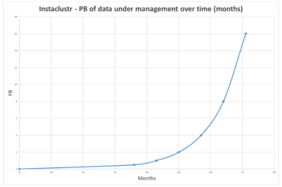
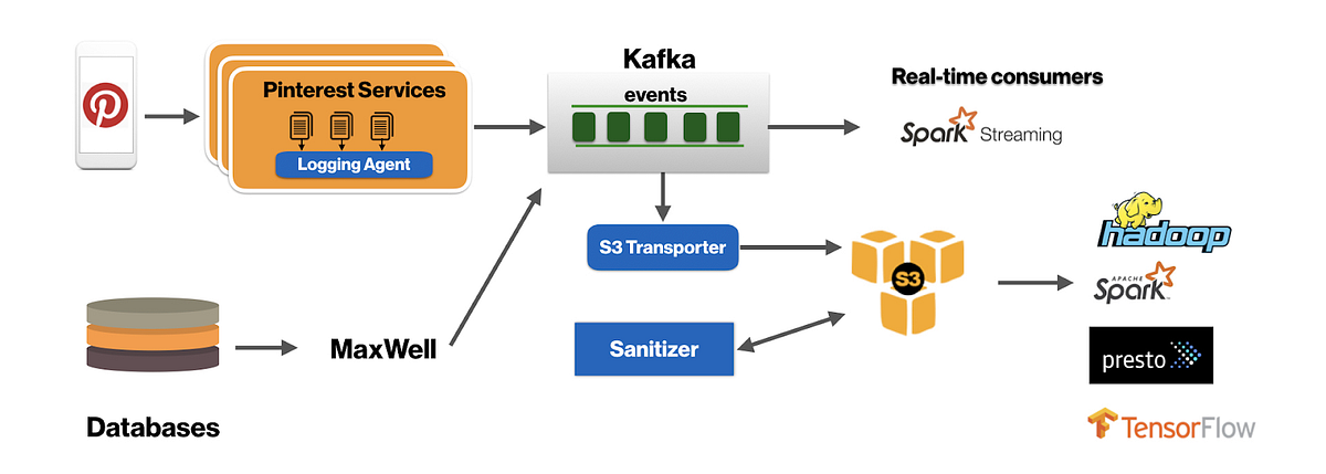
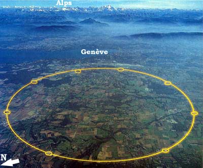
Illustration Image

Sorry about missing last week, but my birthday won out over working: 

Ouch! @john_overholt: My actual life is now a science exhibit about the primitive conditions of the past.

If you like this sort of Stuff then please support me on Patreon.

  • 1PB: SSD in 1U chassis; 90%: savings using EC2 Spot for containers; 16: forms of inertia; $2.1B: Alibaba’s profit; 22.6B: app downloads in Q2; 25%: Google generated internet traffic; 20 by 20 micrometers: quantum random number generators; 16: lectures on Convolutional Neural Networks for Visual Recognition; 25,000: digitized gramophone records; 280%: increase in IoT attacks; 6.5%: world's GDP goes to subsidizing fossil fuel; 832 TB: ZFS on Linux;  $250,000: weekly take from breaking slot machines; 30: galatic message exchanges using artificial megastructures in 100,000 years; 

  • Quotable Quotes:
    • @chris__martin: ALIENS: we bring you a gift of reliable computing technol--

      HUMANS: oh no we have that already but JS is easier to hire for

    • @rakyll: "You woman, you like intern." I interned on F-16's flight computer. Even my internship was 100x more legit than any job you will have.
    • @CodeWisdom: "Debugging is like being the detective in a crime movie where you are also the murderer." - Filipe Fortes
    • William Gibson: what I find far more ominous is how seldom, today, we see the phrase “the 22nd century.” Almost never. Compare this with the frequency with which the 21st century was evoked in popular culture during, say, the 1920s.
    • Arador: Amazon EC2, Microsoft Azure and Google Gloud Platform are all seriously screwing their customers over when it comes to bandwidth charges. Every one of the big three has massive buying power yet between them their average bandwidth price is 3.4x higher than colocation facilities.
    • @mattklein123: Good thread: my view: 1) most infra startups will fail. It's an awful business to be in (sorry all, much ❤️).
    • Jean-Louis Gassée: With Services, Apple enjoys the benefits of a virtuous circle: Hardware sales create Services revenue opportunities; Services makes hardware more attractive and “stickier”. Like Apple Stores, Services are part of the ecosystem. Such is the satisfying simplicity and robustness of Apple’s business model.
    • cardine: The price difference between Hetzner and AWS is large enough that it could pay for 4x as much computational power (as much redundancy as you'd ever need), three full time system admins (not that you'd ever need them), and our office lease... with plenty of money left over!
    • Brujo Benavides: Communication is Key: Have you ever watched a movie or a soap opera and thought “If you would’ve just told her that, we would’ve avoided 3 entire episodes, you moron!”. Happens to me all the time. At Inaka we learned that the hard way.
    • @f3ew: Doesn't matter how many layers of stateless services you have in the middle, the interesting ends have state.
    • brianwawok: My cloud cost is less than 5% of my bussiness costs using GCE. Would be foolish to move it to lower my costs 2%.
    • @f3ew: Stateless services are as relevant as routers. Pattern match, compute, push to next layer.

    • Horace Dediu~ when you outsource you're taking knowledge out of your company, which ends up gutting it in terms of the value that is added 

    • Jason Calacanis: Google was the twelfth search engine. Facebook was the tenth social network. iPad was the twentieth tablet. It’s not who gets there first. It’s who gets there first when the market’s ready.

    • puzzle: The B4 paper states multiple times that Google runs links at almost 100% saturation, versus the standard 30-40%. That's accomplished through the use of SDN technology and, even before that, through strict application of QoS.

    • @stu: Serverless has in many ways eclipsed the containers discussion for the hot buzz in the industry

    • @mjpt777: GC is a wonderful thing but I cannot help but feel it leaves the typical developer even less prepared for distributed resource management.

    • joaodlf: Spark works and does a good job, it has many features that I can see us use in the future too. With that said, it's yet another piece of tech that bloats our stack. I would love to reduce our tech debt: We are much more familiar with relational databases like MySQL and Postgres, but we fear they won't answer the analytics problems we have, hence Cassandra and Spark. We use these technologies out of necessity, not love for them.

    • tobyjsullivan: No, dear author. Setting up the AWS billing alarm was the smartest thing you ever did. It probably saved you tens of thousands of dollars (or at least the headache associated with fighting Amazon over the bill). Developers make mistakes. It's part of the job. It's not unusual or bad in any way. A bad developer is one who denies that fact and fails to prepare for it. A great developer is one like the author.

    • Geoff Wozniak: Regardless of whether I find that stored procedures aren't actually that evil or whether I keep using templated SQL, I do know one thing: I won't fall into the "ORMs make it easy" trap.

    • @BenedictEvans: Part of what distinguishes today’s big tech companies is a continual push against complacency. They saw the last 20 years and read the books

    • John Patrick Pullen: In the upcoming fall issue of Porter magazine, the 21-yer-old X-Men: Apocalypse star said, "I auditioned for a project and it was between me and another girl who is a far better actress than I am, far better, but I had the followers, so I got the job," according to The Telegraph. "It’s not right, but it is part of the movie industry now."

    • Rachel Adler: Naturally, faster prints drove up demand for paper, and soon traditional methods of paper production couldn’t keep up. The paper machine, invented in France in 1799 at the Didot family’s paper mill, could make 40 times as much paper per day as the traditional method, which involved pounding rags into pulp by hand using a mortar and pestle.

    • pawelkomarnicki: As a person that can get the product from scratch to production and scale it, I can say I'm a full-stack developer. Can I feel mythical now?

    • Risto: Before integrating any payment flow make sure you understand the whole flow and the different payment states trialing -> active -> unpaid -> cancelled. For Braintree there is a flow chart. For Stripe there is one too. Both payment providers have REST API’s so make sure to play through the payment flows before starting actual coding.

    • Seyi Fabode: I have 3 neighbors in close proximity who also have solar panels on their roofs. And a couple of other neighbors with electric cars. What says we can’t start our own mini-grid system between ourselves?

    • pixl97: Muscles/limbs are only 'vastly' more efficient if you consider they have large numbers of nano scale support systems constantly rebuilding them. Since we don't have nanobots, gears will be better for machines. Also, nature didn't naturally develop a axle.

    • Brave New Greek: I sympathize with the Go team’s desire to keep the overall surface area of the language small and the complexity low, but I have a hard time reconciling this with the existing built-in generics and continued use of interface{} in the standard library.

    • @jeffhollan: Agree to a point. But where does PaaS become “serverless”? Feel should be ‘infinite’ scale of dynamic allocation of resources + micro bill

    • @kcimc: common tempos in 1M songs, 1959-2011: 120 bpm takes over in the late 80s, and bpms at multiples of 10 emerge in the mid 90s

    • How to Map the Circuits That Define Us: If neural circuits can teach one lesson, it is that no network is too small to yield surprises — or to frustrate attempts at comprehension.

    • @orskov: In Q2, The Wall Street Journal had 1,270,000 daily digital-only subscribers, a 34% increase compared to last year

    • Thrust Zone: A panel including tech billionaire Elon Musk is discussing the fact that technology has progressed so much that it may soon destroy us and they have to pass microphones to talk.

    • @damonedwards: When we are all running containers in public clouds, I’m really going to miss datacenter folks one-upping each other on hardware specs.

    • @BenedictEvans: 186 page telecoms report from 1994. 5 pages on ‘videophones’: no mention of internet. 10 pages saying web will lose to VR. Nothing on mobile

    • Thomas Metzinger: The superintelligence concludes that non-existence is in the own best interest of all future self-conscious beings on this planet. Empirically, it knows that naturally evolved biological creatures are unable to realize this fact because of their firmly anchored existence bias. The superintelligence decides to act benevolently.

    • Jeremy Eder: As with all public cloud, you can do whatever you want…for a price.  BurstBalance is the creation of folks who want you to get hooked on great performance (gp2 can run at 3000+ IOPS), but then when you start doing something more than dev/test and run into these weird issues, you’re already hooked and you have no choice but to pay more for a service that is actually usable.

    • Katz and Fan: After all, the important thing for anyone looking to launder money through a casino isn’t to win. It’s to exchange millions of dollars for chips you can swap for cool, untraceable cash at the end of the night.

    • Caitie McCaffrey: Verification in industry generally consists of unit tests, monitoring, and canaries. While this provides some confidence in the system's correctness, it is not sufficient. More exhaustive unit and integration tests should be written. Tools such as random model checkers should be used to test a large subset of the state space. In addition, forcing a system to fail via fault injection should be more widely used. Even simple tests such as running kill −9 on a primary node have found catastrophic bugs.

    • Zupa: FPGAs give you most of the benefits of special-purpose processors, for a fraction of the cost. They are about 10x slower, but that means an FPGA based bitcoin miner is still 100k times faster than a processor based one

    • menge101work: I'm not sure if the implication is that our CPUs will have gate arrays on chip with the generic CPU, that is an interesting idea. But if they are not on chip, the gate array will never be doing anything in a few clock cycles. It'll be more akin to going out to memory, the latency between a real memory load and an L1 or L2 cache hit is huge. (reference)

      Not to say that being able to do complex work on dedicated hardware won't still be fast, but the difference between on-die and off-die is a huge difference in how big of a change this could be.

    • Animats: This article [Why Many Smart Contract Use Cases Are Simply Impossible] outlines the basic problem. If you want smart contracts that do anything off chain, there have to be connections to trusted services that provide information and take actions. If you have trusted services available, you may not need a blockchain.The article points out that you can't construct an ordinary loan on chain, because you have no way to enforce paying it back short of tying up the loaned funds tor the duration of the loan. Useful credit fundamentally requires some way of making debtors pay up later. It's possible to construct various speculative financial products entirely on chain, and that's been done, but it's mostly useful for gambling, broadly defined.

    • curun1r: Your characterization of startup cloud costs is laughably outdated. With credits for startups and the ability to go serverless, I've known startups that didn't pay a dime for hosting their entire first year despite reaching the threshold of hundreds of customers and over $1m ARR. One of my friends actually started doing some ML stuff on AWS because he wanted to use his remaining credits before they expired and his production and staging workloads weren't going to get him there. I'd say it makes no sense to buy your 32gb, 16-core single point of fail, waste $40/mo and half a day setting it up and then have to keep it running yourself when you can easily spin up an API in API Gateway/Lambda that dumps data into dynamo/simpledb and front it with a static site in S3. That setup scales well enough to be mentioned on HN without getting hugged to death and is kept running by someone else. And if it is, literally, free for the first year, how is that not a no brainer?

    • Neil Irwin: In this way of thinking about productivity, inventors and business innovators are always cooking up better ways to do things, but it takes a labor shortage and high wages to coax firms to deploy the investment it takes to actually put those innovations into widespread use. In other words, instead of worrying so much about robots taking away jobs, maybe we should worry more about wages being too low for the robots to even get a chance.

Don't miss all that the Internet has to say on Scalability, click below and become eventually consistent with all scalability knowledge (which means this post has many more items to read so please keep on reading)...

1. Hello, World!

Hi, I’m Paul Brebner and this is a “Hello, World!” blog to introduce myself and test everything out. I’m very excited to have started at Instaclustr last week as a Technology Evangelist.   

One of the cool things to happen in my first week was that Instaclustr celebrated a significant milestone when it exceeded 1 Petabyte (1PB) of data under management.  Is this a lot of data? Well, yes! A Petabyte is 10^15 bytes, 1 Quadrillion bytes (which sounds more impressive!), or 1,000,000,000,000,000 bytes.

Also, I’m a Petabyte Person. Apart from my initials being PB, the human brain was recently estimated to have 1PB of storage capacity, not bad for a 1.4kg meat computer! So in this post, I’m going to introduce myself and some of what I’ve learned about Instaclustr by exploring what that Petabyte means.

Folklore has it that the 1st “Hello, World!” program was written in BCPL (the programming language that led to C), which I used to program a 6809 microprocessor I built in the early 1980’s. In those days the only persistent storage I had were 8-inch floppy disks. Each disk could hold 1MB of data, so you’d need 10^9 (1,000,000,000) 8-inch floppy disks to hold 1PB of data.  That’s a LOT of disks, and would weigh a whopping 31,000 tonnes, as much as the German WWII Pocket Battleship the Admiral Graf Spee.

the German WWII Pocket Battleship the Admiral Graf Spee

Source: Wikipedia

1PB of data is also a lot in terms of my experience.  I worked in R&D for CSIRO and UCL in the areas of middleware, distributed systems, grid computing, and sensor networks etc between 1996-2007. During 2003 I was the software architect for a CSIRO Grid cluster computing project with Big Astronomy Data – all 2TB of it. 1PB is 500,000 times more data than that.

What do Instaclustr and the Large Hadron Collider have in common?

Large Hadron Collider Instaclustr

Source: cms.cern

Apart from the similarity of the Instaclustr Logo and the aerial shot of the LHC? (The circular pattern)

LHC from above

Instaclustr logo & the Large Hadron Collider

Source: Sequim Science

The LHC “Data Centre processes about one petabyte of data every day“.  More astonishing is that the LHC has a huge number of detectors which spit out data at the astonishing rate of 1PB/s – most of which they don’t (and can’t) store.

2. Not just Data Size

But there’s more to data than just the dimension of size. There are large amounts of “dead” data lying around on archival storage media which is more or less useless. But live dynamic data is extremely useful and is of enormous business value. So apart from being able to store 1PB of data (and more), you need to be able to: write data fast enough, keep track of what data you have, find the data and use it, have 24×7 availability, and have sufficient processing and storage capacity on-demand to do useful things as fast as possible (scalability and elasticity).  How is this possible? Instaclustr!

The Instaclustr value proposition is: “Reliability at scale.”

Instaclustr solves the problem of “reliability at scale” via a combination of Scalable Open Source Big Data technologies, Public Cloud hosting, and Instaclustr’s own Managed Services technologies (including cloud provisioning, cluster monitoring and management, automated repairs and backups, performance optimization, scaling and elasticity).

How does this enable reliability at Petabyte data scale? Here’s just one example. If you have 1PB+ of data on multiple SSDs in your own data centre an obvious problem would be data durability.  1PB is a lot of data, and SSDs are NOT 100% error free (the main problem is “quantum tunneling” which “drills holes” in SSDs and imposes a maximum number of writes).  These people did the experiment to see how many writes it took before different SSDs died, and the answer is in some cases it’s less than 1PB. So, SSDs will fail and you will lose data – unless you have taken adequate precautions and continue to do so. The whole system must be designed and operated assuming failure is normal.

The Cassandra NoSQL database itself is designed for high durability by replicating data on as many different nodes as you specify (it’s basically a shared-nothing P2P distributed system).  Instaclustr enhances this durability by providing automatic incremental backups (to S3 on AWS), multiple region deployments for AWS, automated repairs, and 24×7 monitoring and management.

3. The Data Network Effect

1PB of data under management by Instaclustr is a noteworthy milestone, but that’s not the end of the story. The amount of data will GROW! The Network effect is what happens when the value of a product or service increases substantially with the number of other people using it. The classic example is the telephone system.  A single telephone is useless, but 100 telephones connected together (even manually by an operator!) is really useful, and so the network grows rapidly.  Data Network effects are related to the amount and interconnectedness of data in a system.  

For Instaclustr customers the Data Network effect is likely to be felt in two significant ways.  Firstly, the amount of data customers have in their Cassandra cluster will increase – as it increases over time the value will increase significantly; also velocity: the growth of data, services, sensors and applications in the related ecosystems – e.g in the AWS ecosystem – will accelerate.  Secondly, the continued growth in clusters and data under management provides considerable more experience, learned knowledge and capabilities for managing your data and clusters.

Here’s a prediction. I’ve only got 3 data points to go on. When Instaclustr started (in 2014) it was managing 0PB of data. At the end of 2016 this had increased to 0.5PB, and in July 2017 we reached 1PB. Assuming the amount of data continues to double at the same rate in the future, then the total data under management by Instaclustr may increase massively over the next 3 years

Graph of months vs PB Data Instaclustr

(Graph of Months vs PB of data).

4. What next?

I started as Technology Evangelist at Instaclustr (last week). My background for the last 10 years has been a senior research scientist in NICTA (National ICT Australia, now merged with CSIRO as Data61), and for the last few years at CTO/consultant with a NICTA start-up specializing in performance engineering (via Performance Data Analytics and Modelling). I’ve invented some performance analytics techniques, commercialized them in a tool, and applied them to client problems, often in the context of Big Data Analytics problems. The tool we developed actually used Cassandra (but in a rather odd way, we needed to store very large volumes of performance data for later analysis from a simulation engine, hours of data could be simulated and needed to be persisted in a few seconds and Cassandra was ideal for that use case). I’m also an AWS Associate Solution Architect. Before all this, I was a Computer Scientist, Machine Learning researcher, Software Engineer, Software Architect, UNIX systems programmer, etc.  Some of this may come in useful for getting up to speed with Cassandra etc.

Over the next few months, the plan is for me to understand the Instaclustr technologies from “end user” and developer perspectives, develop and try out some sample applications, and blog about them. I’m going to start with the internal Instaclustr use case for Cassandra, which is the heart of the performance data monitoring tool (Instametrics).  Currently there’s lots of performance data stored in Cassandra, but only a limited amount of analysis and prediction being done (just aggregation). It should be feasible and an interesting learning exercise to do some performance analytics on the Cassandra data performance data to predict interesting events in advance and take remedial action.

I’m planning to start out with some basic use cases and programming examples for Cassandra (e.g. how do you connect to Cassandra, how do you find out what’s in it, how do get data out of it, how do you do simple queries such as finding “outliers”, how do you more complex Data Analytics (e.g. regression analysis, ML, etc), etc. I’ll probably start out very simple. e.g. Cassandra & Java on my laptop, having a look at some sample Cassandra data, try some simple Data analytics, then move to more complex examples as the need arises. E.g. Cassandra on Instaclustr, Java on AWS, Spark + MLLib, etc. I expect to make some mistakes and revise things as I go. Most of all I hope to make it interesting.

Watch this space ????

The post Paul Brebner (the Petabyte Person) joins Instaclustr (the Petabyte Company) appeared first on Instaclustr.

A handy feature was silently added to Apache Cassandra’s nodetool just over a year ago. The feature added was the -j (jobs) option. This little gem controls the number of compaction threads to use when running either a scrub, cleanup, or upgradesstables. The option was added to nodetool via CASSANDRA-11179 to version 3.5. It has been back ported to Apache Cassandra versions 2.1.14, 2.2.6, and 3.5.

If unspecified, nodetool will use 2 compaction threads. When this value is set to 0 all available compaction threads are used to perform the operation. Note that the total number of available compaction threads is controlled by the concurrent_compactors property in the cassandra.yaml configuration file. Examples of how it can be used are as follows.

$ nodetool scrub -j 3
$ nodetool cleanup -j 1
$ nodetool upgradesstables -j 1 

The option is most useful in situations where disk space is scarce and a limited number of threads for the operation need to be used to avoid disk exhaustion.

Introduction I’ve wanted to create a system which in its core uses event sourcing for quite a while - actually since I’ve read Martin Kleppmann’s Making Sense of Stream Processing. The book is really amazing, Martin tends to explain all concepts from basic building blocks and in a really simple and understandable way. I recommend it to everyone. The idea is to have a running Cassandra cluster and to evolve a system with no downtime in such a way that Kafka is the Source of Truth with immutable facts. Every other system (in this case Cassandra cluster) should use these facts and aggregate / transform them for its purpose. Also, since all facts are in Kafka, it should be easy to drop the whole database, index, cache or any other data system and recreate it from scratch again. The following diagrams should illustrate the system evolution. Starting system architecture   Target system architecture   When observing the diagrams, it seems like a pretty straightforward and trivial thing to do, but there’s more to it, especially when you want to do it with no downtime. Evolution breakdown I tried to break down the evolution process to a few conceptual steps and this is what I came up with: Have a mechanism to push each Cassandra change to Kafka with timestamp Start collecting each Cassandra change to temporary Kafka topic I need to start collecting before a snapshot is taken, otherwise there will be a time window in which incoming changes would be lost, and it also needs to go to temporary topic since there is data in the database which should be first in an ordered sequence of events Take the existing database snapshot This one is pretty straightforward Start reading data from the snapshot into the right Kafka topic Since the data from the snapshot was created first, it should be placed first into Kafka After the snapshot is read, redirect the data from the temporary Kafka topic to the right Kafka topic, but mind the timestamp when the snapshot is taken This step is essential to be done correctly, and could be considered as the hardest part. Since change event collecting started before the snapshot, there is a possibility that some events also exist in the snapshot as well and, to avoid inconsistencies, each event should be idempotent and I should try to be as precise as possible when comparing the event timestamp with the snapshot timestamp Create a new Cassandra cluster/keyspace/table and Kafka stream to read from Kafka and insert into this new Cassandra cluster/keyspace/table As a result, the new cassandra cluster should be practically a copy/clone of the existing one Wait for the temporary Kafka topic to deplete If I change the application to read from the new cassandra right away, and Kafka temporary topic still doesn’t catch up with system, there will be significant read delays (performance penalties) in the system. To make sure everything is in order, I think monitoring of time to propagate the change to the new Cassandra cluster will help and if the number is decent (a few milliseconds), I can proceed to the next step Change the application to read from the new cassandra instead of old and still write to old Since everything is done within the no downtime context, the application is actually several instances of application on different nodes, and they won’t be changed simultaneously, that would cause the downtime. I’d need to change one at a time, while others are still having the old software version. For this reason, the application still needs to write to the old cassandra, since other application nodes are still reading from the old cassandra. When each application instance is updated, change the application to write directly to Kafka right topic Now each node, one by one, can be updated with new application version which will write directly to Kafka. In parallel, old nodes will write to the old Cassandra which will propagate to Kafka topic, and new nodes will write directly to the Kafka topic. When the change is complete, all nodes are writing directly to the Kafka topic and we are good to go. Clean up At this point, the system writes to the right Kafka topic, the stream is reading from it and making inserts into the new Cassandra. The old Cassandra and Kafka temporary topic are no longer necessary so it should be safe for me to remove them. Well, that’s the plan, so we’ll see whether it is doable or not. There are a few motivating factors why I’ve chosen to evolve an existing system instead of building one the way I want from scratch. It is more challenging, hence more fun The need for evolving existing systems is the everyday job of software developers; you don’t get a chance to build a system for a starting set of requirements with guarantee that nothing in it will ever change (except for a college project, perhaps) When a system needs to change, you can choose two ways, to build a new one from scratch and when ready replace the old or to evolve the existing. I’ve done the former a few times in my life, and it might seem as fun at the beginning, but it takes awfully long, with a lot of bug fixing, often ends up as a catastrophe and is always expensive Evolving a system takes small changes with more control, instead of placing a totally new system instead of the old. I’m a fan of Martin Fowler’s blog, Evolutionary Database Design fits particularly nicely in this topic Since writing about this in a single post would render quite a huge post, I’ve decided to split it into a few, I’m still not sure how many, but I’ll start and see where it takes me. Bear with me. Data model I’ll start with data model. Actually, it is just one simple table, but it should be enough to demonstrate the idea. The following CQL code describes the table. CREATE TABLE IF NOT EXISTS movies_by_genre (title text,genre text,year int,rating float,duration int,director text,country text,PRIMARY KEY ((genre, year), rating, duration)) WITH CLUSTERING ORDER BY (rating DESC, duration ASC) The use case for this table might not be that common, since the table is actually designed to have a complex primary key with at least two columns as a partition key and at least two clustering columns. The reason for that is it will leverage examples, since handling of a complex primary key might be needed for someone reading this. In order to satisfy the first item from the Evolution breakdown, I need a way to push each Cassandra change to Kafka with a timestamp. There are a few ways to do it: Cassandra Triggers, Cassandra CDC, Cassandra Custom Secondary Index and possibly some other ways, but I’ll investigate only the three mentioned. Cassandra Triggers For this approach I’ll use two Cassandra 3.11.0 nodes, two Kafka 0.10.1.1 nodes and one Zookeeper 3.4.6. Every node will run in a separate Docker container. I decided to use Docker since it keeps my machine clean and it is easy to recreate infrastructure. To create a trigger in Cassandra, ITrigger interface needs to be implemented. The interface itself is pretty simple: public interface ITrigger {public Collection<Mutation> augment(Partition update);} And that’s all there is to it. The interface has been changed since Cassandra 3.0. Earlier versions of Cassandra used the following interface: public interface ITrigger {public Collection<Mutation> augment(ByteBuffer partitionKey, ColumnFamily update);} Before I dive into implementation, let’s discuss the interface a bit more. There are several important points regarding the implementation that need to be honored and those points are explained on the interface’s javadoc: Implementation of this interface should only have a constructor without parameters ITrigger implementation can be instantiated multiple times during the server life time. (Depends on the number of times the trigger folder is updated.) ITrigger implementation should be stateless (avoid dependency on instance variables). Besides that, augment method is called exactly once per update and Partition object contains all relevant information about the update. You might notice that return type is not void but rather a collection of mutations. This way trigger can be implemented to perform some additional changes when certain criteria are met. But since I just want to propagate data to Kafka, I’ll just read the update information, send it to Kafka and return empty mutation collection. In order not to pollute this article with a huge amount of code, I’ve created maven project which creates a JAR file, and the project can be found here. I’ll try to explain the code in the project. Firstly, there is a FILE_PATH constant, which points to /etc/cassandra/triggers/KafkaTrigger.yml and this is where YAML configuration for trigger class needs to be. It should contain configuration options for Kafka brokers and for topic name. The file is pretty simple, since the whole file contains just the following two lines: bootstrap.servers: cluster_kafka_1:9092,cluster_kafka_2:9092 topic.name: trigger-topic I’ll come to that later when we build our docker images. Next, there is a constructor which initializes the Kafka producer and ThreadPoolExecutor. I could have done it without ThreadPoolExecutor, but the reason for it is that the trigger augment call is on Cassandra’s write path and in that way it impacts Cassandra’s write performances. To minimize that, I’ve moved trigger execution to background thread. This is doable in this case, since I am not making any mutations, I can just start the execution in another thread and return an empty list of mutations immediately. In case when the trigger needs to make a mutation based on partition changes, that would need to happen in the same thread. Reading data from partition update in augment method is really a mess. Cassandra API is not that intuitive and I went through a real struggle to read all the necessary information. There are a few different ways to update a partition in Cassandra, and these are ones I’ve covered: Insert Update Delete of director column Delete of title column Delete of both director and title columns Delete of row Delete range of rows for last clustering column (duration between some values) Delete all rows for specific rating clustering column Delete range of rows for first clustering column (rating between some values) Delete whole partition A simplified algorithm would be: if (isPartitionDeleted(partition)) {handle partition delete;} else {if (isRowUpdated(partition)) {if (isRowDeleted(partition)) {handle row delete;} else {if (isCellDeleted(partition)) {handle cell delete;} else {handle upsert;}}} else if (isRangeDelete(partition)) {handle range delete;}} In each case, JSON is generated and sent to Kafka. Each message contains enough information to recreate Cassandra CQL query from it. Besides that, there are a few helper methods for reading the YAML configuration and that is all. In order to test everything, I’ve chosen Docker, as stated earlier. I’m using Cassandra docker image with 3.11.0 tag. But since the JAR file and KafkaTrigger.yml need to be copied into the docker container, there are two options: Use Cassandra 3.11.0 image and docker cp command to copy the files into the container Create a new Docker image with files already in it and use that image The first option is not an option actually, it is not in the spirit of Docker to do such thing so I will go with the second option. Create a cluster directory somewhere and a cassandra directory within it mkdir -p cluster/cassandra cluster directory will be needed for later, now just create KafkaTrigger.yml in cassandra dir with the content I provided earlier. Also, the built JAR file (cassandra-trigger-0.0.1-SNAPSHOT.jar) needs to be copied here. To build all that into Docker, I created a Dockerfile with the following content: FROM cassandra:3.11.0COPY KafkaTrigger.yml /etc/cassandra/triggers/KafkaTrigger.ymlCOPY cassandra-trigger-0.0.1-SNAPSHOT.jar /etc/cassandra/triggers/trigger.jarCMD ["cassandra", "-f"] In console, just position yourself in the cassandra directory and run: docker build -t trigger-cassandra . That will create a docker image with name trigger-cassandra. All that is left is to create a Docker compose file, join all together and test it. The Docker compose file should be placed in the  cluster directory. The reason for that is because Docker compose has a naming convention for containers it creates, it is <present_directory_name>_<service_name>_<order_num>. And I already specified the Kafka domain names in KafkaTrigger.yml as cluster_kafka_1 and cluster_kafka_2, in case the Docker compose is run from another location, container naming would change and KafkaTrigger.yml would need to be updated. My Docker compose file is located in the cluster directory, it’s named cluster.yml and it looks like this: version: '3.3'services:zookeeper:image: wurstmeister/zookeeper:3.4.6ports:- "2181:2181"kafka:image: wurstmeister/kafka:0.10.1.1ports:- 9092environment:HOSTNAME_COMMAND: "ifconfig | awk '/Bcast:.+/{print $$2}' | awk -F\":\" '{print $$2}'"KAFKA_ADVERTISED_PORT: 9092KAFKA_ZOOKEEPER_CONNECT: zookeeper:2181cassandra-seed:image: trigger-cassandraports:- 7199- 9042environment:CASSANDRA_CLUSTER_NAME: test-clustercassandra:image: trigger-cassandraports:- 7199- 9042environment:CASSANDRA_CLUSTER_NAME: test-clusterCASSANDRA_SEEDS: cassandra-seed The cluster contains the definition for Zookeeper, Kafka and Cassandra with the exception that there are two Cassandra services. The reason for that is that one can be standalone, but all others need a seed list. cassandra-seed will serve as seed, and cassandra as scalable service. That way, I can start multiple instances of cassandra. However, to start multiple instances, it takes time, and it is not recommended to have multiple Cassandra nodes in joining state. So, scale should be done one node at a time. That does not apply to Kafka nodes. With the following command, I’ve got a running cluster ready for use: docker-compose -f cluster.yml up -d --scale kafka=2 After that, I connected to the Cassandra cluster with cqlsh and created the keyspace and table. To add a trigger to the table, you need to execute the following command: CREATE TRIGGER kafka_trigger ON movies_by_genre USING 'io.smartcat.cassandra.trigger.KafkaTrigger'; In case you get the following error: ConfigurationException: Trigger class 'io.smartcat.cassandra.trigger.KafkaTrigger' doesn't exist There are several things that can be wrong. The JAR file might not be loaded within the Cassandra node; that should happen automatically, but if it doesn’t you can try to load it with: nodetool reloadTriggers If the problem persists, it might be that the configuration file is not at a proper location, but that can only happen if you are using a different infrastructure setup and you forgot to copy KafkaTrigger.yml to the proper location. Cassandra will show the same error even if class is found but there is some problem instantiating it or casting it to theITrigger interface. Also, make sure that you implemented the ITrigger interface from the right Cassandra version (versions of cassandra in the JAR file and of the cassandra node should match). If there are no errors, the trigger is created properly. This can be checked by executing the following CQL commands: USE system_schema;SELECT * FROM triggers; Results I used kafka-console-consumer to see if messages end up in Kafka, but any other option is good enough. Here are a few things I tried and the results it gave me. For most cases, not all of these mutations are used, usually it’s just insert, update and one kind of delete. Here I intentionally tried several ways since it might come in handy to someone. In case you have a simpler table use case, you might be able to simplify the trigger code as well. What is also worth noting is that triggers execute only on a coordinator node; they have nothing to do with data ownership nor replication and the JAR file needs to be on every node that can become a coordinator. Going a step further This is OK for testing purposes, but for this experiment to have any value, I will simulate the mutations to the cassandra cluster at some rate. This can be accomplished in several ways, writing a custom small application, using cassandra stress or using some other tool. Here at SmartCat, we have developed a tool for such purpose. That is the easiest way for me to create load on a Cassandra cluster. The tool is called Berserker, you can give it a try. To start with Berserker, I’ve downloaded the latest version (0.0.7 is the latest at the moment of writing) from here. And I’ve created a configuration file named configuration.yml. load-generator-configuration section is used to specify all other configurations. There, for every type of the configuration, name is specified in order for the Berserker to know which configuration parser to use in concrete sections. After that, a section for each configuration with parser specific options and format is found. There are following sections available: data-source-configuration where data source which will generate data for worker is specified rate-generator-configuration where should be specified how rate generator will be created and it will generate rate. This rate is rate at which worker will execute worker-configuration, configuration for worker metrics-reporter-configuration, configuration for metrics reporting, currently only JMX and console reporting is supported In this case, the data-source-configuration section is actually a Ranger configuration format and can be found here. An important part for this article is the connection-points property within worker-configration. This will probably be different every time Docker compose creates a cluster. To see your connection points run: docker ps It should give you a similar output: There you can find port mapping for cluster_cassandra-seed_1 and cluster_cassandra_1 containers and use it, in this case it is: 0.0.0.0:32779 and 0.0.0.0:32781. Now that everything is settled, just run: java -jar berserker-runner-0.0.7.jar -c configuration.yml Berserker starts spamming the Cassandra cluster and in my terminal where kafka-console-consumer is running, I can see messages appearing, it seems everything is as expected, at least for now. End That’s all, next time I’ll talk about Cassandra CDC and maybe custom secondary index. Hopefully, in a few blog posts, I’ll have the whole idea tested and running.

One of the common griefs Scala developers express when using the DataStax Java driver is the overhead incurred in almost every read or write operation, if the data to be stored or retrieved needs conversion from Java to Scala or vice versa.

This could be avoided by using "native" Scala codecs. This has been occasionally solicited from the Java driver team, but such codecs unfortunately do not exist, at least not officially.

Thankfully, the TypeCodec API in the Java driver can be easily extended. For example, several convenience Java codecs are available in the driver's extras package.

In this post, we are going to piggyback on the existing extra codecs and show how developers can create their own codecs – directly in Scala.

Note: all the examples in this post are available in this Github repository.

Dealing with Nullability

It can be tricky to deal with CQL types in Scala because CQL types are all nullable, whereas most typical representations of CQL scalar types in Scala resort to value classes, and these are non-nullable.

As an example, let's see how the Java driver deserializes, say, CQL ints.

The default codec for CQL ints converts such values to java.lang.Integer instances. From a Scala perspective, this has two disadvantages: first, one needs to convert from java.lang.Integer to Int, and second, Integer instances are nullable, while Scala Ints aren't.

Granted, the DataStax Java driver's Row interface has a pair of methods named getInt that deserialize CQL ints into Java ints, converting null values into zeroes.

But for the sake of this demonstration, let's assume that these methods did not exist, and all CQL ints were being converted into java.lang.Integer. Therefore, developers would yearn to have a codec that could deserialize CQL ints into Scala Ints while at the same time addressing the nullability issue.

Let this be the perfect excuse for us to introduce IntCodec, our first Scala codec:

import java.nio.ByteBuffer
import com.datastax.driver.core.exceptions.InvalidTypeException
import com.datastax.driver.core.{DataType, ProtocolVersion, TypeCodec}
import com.google.common.reflect.TypeToken
object IntCodec extends TypeCodec[Int](DataType.cint(), TypeToken.of(classOf[Int]).wrap()) {
  override def serialize(value: Int, protocolVersion: ProtocolVersion): ByteBuffer = 
    ByteBuffer.allocate(4).putInt(0, value)
  override def deserialize(bytes: ByteBuffer, protocolVersion: ProtocolVersion): Int = {
    if (bytes == null || bytes.remaining == 0) return 0
    if (bytes.remaining != 4) throw new InvalidTypeException("Invalid 32-bits integer value, expecting 4 bytes but got " + bytes.remaining)
    bytes.getInt(bytes.position)
  }
  override def format(value: Int): String = value.toString
  override def parse(value: String): Int = {
    try {
      if (value == null || value.isEmpty || value.equalsIgnoreCase("NULL")) 0
      else value.toInt
    }
    catch {
      case e: NumberFormatException =>
        throw new InvalidTypeException( s"""Cannot parse 32-bits integer value from "$value"""", e)
    }
  }
}

All we did so far is extend TypeCodec[Int] by filling in the superclass constructor arguments (more about that later) and implementing the required methods in a very similar way compared to the driver's built-in codec.

Granted, this isn't rocket science, but it will get more interesting later. The good news is, this template is reproducible enough to make it easy for readers to figure out how to create similar codecs for every AnyVal that is mappable to a CQL type (Boolean, Long, Float, Double, etc... let your imagination run wild or just go for the ready-made solution).

(Tip: because of the automatic boxing/unboxing that occurs under the hood, don't use this codec to deserialize simple CQL ints, and prefer instead the driver's built-in one, which will avoid this overhead; but you can use IntCodec to compose more complex codecs, as we will see below – the more complex the CQL type, the more negligible the overhead becomes.)

Let's see how this piece of code solves our initial problems: as for the burden of converting between Scala and Java, Int values are now written directly with ByteBuffer.putInt, and read directly from ByteBuffer.getInt; as for the nullability of CQL ints, the issue is addressed just as the driver does: nulls are converted to zeroes.

Converting nulls into zeroes might not be satisfying for everyone, but how to improve the situation? The general Scala solution for dealing with nullable integers is to map them to Option[Int]. DataStax Spark Connector for Apache Cassandra®'s CassandraRow class has exactly one such method:

def getIntOption(index: Int): Option[Int] = ...

Under the hood, it reads a java.lang.Integer from the Java driver's Row class, and converts the value to either None if it's null, or to Some(value), if it isn't.

Let's try to achieve the same behavior, but using the composite pattern: we first need a codec that converts from any CQL value into a Scala Option. There is no such built-in codec in the Java driver, but now that we are codec experts, let's roll our own OptionCodec:

class OptionCodec[T](
    cqlType: DataType,
    javaType: TypeToken[Option[T]],
    innerCodec: TypeCodec[T])
  extends TypeCodec[Option[T]](cqlType, javaType)
    with VersionAgnostic[Option[T]] {
  def this(innerCodec: TypeCodec[T]) {
    this(innerCodec.getCqlType, TypeTokens.optionOf(innerCodec.getJavaType), innerCodec)
  }
  override def serialize(value: Option[T], protocolVersion: ProtocolVersion): ByteBuffer =
    if (value.isEmpty) OptionCodec.empty.duplicate else innerCodec.serialize(value.get, protocolVersion)
  override def deserialize(bytes: ByteBuffer, protocolVersion: ProtocolVersion): Option[T] =
    if (bytes == null || bytes.remaining() == 0) None else Option(innerCodec.deserialize(bytes, protocolVersion))
  override def format(value: Option[T]): String =
    if (value.isEmpty) "NULL" else innerCodec.format(value.get)
  override def parse(value: String): Option[T] =
    if (value == null || value.isEmpty || value.equalsIgnoreCase("NULL")) None else Option(innerCodec.parse(value))
}
object OptionCodec {
  private val empty = ByteBuffer.allocate(0)
  def apply[T](innerCodec: TypeCodec[T]): OptionCodec[T] =
    new OptionCodec[T](innerCodec)
  import scala.reflect.runtime.universe._
  def apply[T](implicit innerTag: TypeTag[T]): OptionCodec[T] = {
    val innerCodec = TypeConversions.toCodec(innerTag.tpe).asInstanceOf[TypeCodec[T]]
    apply(innerCodec)
  }
}

And voilà! As you can see, the class body is very simple (its companion object is not very exciting at this point either, but we will see later how it could do more than just mirror the class constructor). Its main purpose when deserializing/parsing is to detect CQL nulls and return None right away, without even having to interrogate the inner codec, and when serializing/formatting, intercept None so that it can be immediately converted back to an empty ByteBuffer (the native protocol's representation of null).

We can now combine our two codecs together, IntCodec and OptionCodec, and compose a TypeCodec[Option[Int]]:

import com.datastax.driver.core._
val codec: TypeCodec[Option[Int]] = OptionCodec(IntCodec)
assert(codec.deserialize(ByteBuffer.allocate(0), ProtocolVersion.V4).isEmpty)
assert(codec.deserialize(ByteBuffer.allocate(4), ProtocolVersion.V4).isDefined)

The problem with TypeTokens

Let's sum up what we've got so far: a TypeCodec[Option[Int]] that is the perfect match for CQL ints. But how to use it?

There is nothing really particular with this codec and it is perfectly compatible with the Java driver. You can use it explicitly, which is probably the simplest way:

import com.datastax.driver.core._
val codec: TypeCodec[Option[Int]] = OptionCodec(IntCodec)
val row: Row = ??? // some CQL query containing an int column
val v: Option[Int] = row.get(0, codec)

But your application is certainly more complex than that, and you would like to register your codec beforehand so that it gets transparently used afterwards:

import com.datastax.driver.core._
// first
val codec: TypeCodec[Option[Int]] = OptionCodec(IntCodec)
cluster.getConfiguration.getCodecRegistry.register(codec)
// then
val row: Row = ??? // some CQL query containing an int column
val v: Option[Int] = row.get(0, ???) // How to get a TypeToken[Option[Int]]?

Well, before we can actually do that, we first need to solve one problem: the Row.get method comes in a few overloaded flavors, and the most flavory ones accept a TypeToken argument; let's learn how to use them in Scala.

The Java Driver API, for historical reasons — but also, let's be honest, due to the lack of alternatives – makes extensive usage of Guava's TypeToken API (if you are not familiar with the type token pattern you might want to stop and read about it first).

Scala has its own interpretation of the same reflective pattern, named type tags. Both APIs pursue identical goals – to convey compile-time type information to the runtime – through very different roads. Unfortunately, it's all but an easy path to travel from one to the other, simply because there is no easy bridge between java.lang.Type and Scala's Type.

Hopefully, all is not lost. As a matter of fact, creating a full-fledged conversion service between both APIs is not a pre-requisite: it turns out that Guava's TypeToken works pretty well in Scala, and most classes get resolved just fine. TypeTokens in Scala are just a bit cumbersome to use, and quite error-prone when instantiated, but that's something that a helper object can facilitate.

We are not going to dive any deeper in the troubled waters of Scala reflection (well, at least not until the last chapter of this tutorial). It suffices to assume that the helper object we mentioned above really exists, and that it does the job of creating TypeToken instances while at the same time sparing the developer the boiler-plate code that this operation usually incurs.

Now we can resume our example and complete our code that reads a CQL int into a Scala Option[Int], in the most transparent way:

import com.datastax.driver.core._
val tt = TypeTokens.optionOf(TypeTokens.int) // creates a TypeToken[Option[Int]]
val row: Row = ??? // some CQL query containing an int column
val v: Option[Int] = row.get(0, tt) 

Dealing with Collections

Another common friction point between Scala and the Java driver is the handling of CQL collections.

Of course, the driver has built-in support for CQL collections; but obviously, these map to typical Java collection types: CQL list maps to java.util.List (implemented by java.util.ArrayList), CQL set to java.util.Set (implemented by java.util.LinkedHashSet) and CQL map to java.util.Map (implemented by java.util.HashMap).

This leaves Scala developers with two inglorious options:

  1. Use the implicit JavaConverters object and deal with – gasp! – mutable collections in their code;
  2. Deal with custom Java-to-Scala conversion in their code, and face the consequences of conversion overhead (this is the choice made by the already-mentioned Spark Connector for Apache Cassandra®, because it has a very rich set of converters available).

All of this could be avoided if CQL collection types were directly deserialized into Scala immutable collections.

Meet SeqCodec, our third Scala codec in this tutorial:

import java.nio.ByteBuffer
import com.datastax.driver.core.CodecUtils.{readSize, readValue}
import com.datastax.driver.core._
import com.datastax.driver.core.exceptions.InvalidTypeException
class SeqCodec[E](eltCodec: TypeCodec[E])
  extends TypeCodec[Seq[E]](
    DataType.list(eltCodec.getCqlType),
    TypeTokens.seqOf(eltCodec.getJavaType))
    with ImplicitVersion[Seq[E]] {
  override def serialize(value: Seq[E], protocolVersion: ProtocolVersion): ByteBuffer = {
    if (value == null) return null
    val bbs: Seq[ByteBuffer] = for (elt <- value) yield {
      if (elt == null) throw new NullPointerException("List elements cannot be null")
      eltCodec.serialize(elt, protocolVersion)
    }
    CodecUtils.pack(bbs.toArray, value.size, protocolVersion)
  }
  override def deserialize(bytes: ByteBuffer, protocolVersion: ProtocolVersion): Seq[E] = {
    if (bytes == null || bytes.remaining == 0) return Seq.empty[E]
    val input: ByteBuffer = bytes.duplicate
    val size: Int = readSize(input, protocolVersion)
    for (_ <- 1 to size) yield eltCodec.deserialize(readValue(input, protocolVersion), protocolVersion)
  }
  override def format(value: Seq[E]): String = {
    if (value == null) "NULL" else '[' + value.map(e => eltCodec.format(e)).mkString(",") + ']'
  }
  override def parse(value: String): Seq[E] = {
    if (value == null || value.isEmpty || value.equalsIgnoreCase("NULL")) return Seq.empty[E]
    var idx: Int = ParseUtils.skipSpaces(value, 0)
    if (value.charAt(idx) != '[') throw new InvalidTypeException( s"""Cannot parse list value from "$value", at character $idx expecting '[' but got '${value.charAt(idx)}'""")
    idx = ParseUtils.skipSpaces(value, idx + 1)
    val seq = Seq.newBuilder[E]
    if (value.charAt(idx) == ']') return seq.result
    while (idx < value.length) {
      val n = ParseUtils.skipCQLValue(value, idx)
      seq += eltCodec.parse(value.substring(idx, n))
      idx = n
      idx = ParseUtils.skipSpaces(value, idx)
      if (value.charAt(idx) == ']') return seq.result
      if (value.charAt(idx) != ',') throw new InvalidTypeException( s"""Cannot parse list value from "$value", at character $idx expecting ',' but got '${value.charAt(idx)}'""")
      idx = ParseUtils.skipSpaces(value, idx + 1)
    }
    throw new InvalidTypeException( s"""Malformed list value "$value", missing closing ']'""")
  }
  override def accepts(value: AnyRef): Boolean = value match {
    case seq: Seq[_] => if (seq.isEmpty) true else eltCodec.accepts(seq.head)
    case _ => false
  }
}
object SeqCodec {
  def apply[E](eltCodec: TypeCodec[E]): SeqCodec[E] = new SeqCodec[E](eltCodec)
}

(Of course, we are talking here about scala.collection.immutable.Seq.)

The code above is still vaguely ressemblant to the equivalent Java code, and not very interesting per se; the parse method in particular is not exactly a feast for the eyes, but there's little we can do about it.

In spite of its modest body, this codec allows us to compose a more interesting TypeCodec[Seq[Option[Int]]] that can convert a CQL list<int> directly into a scala.collection.immutable.Seq[Option[Int]]:

import com.datastax.driver.core._
type Seq[+A] = scala.collection.immutable.Seq[A]
val codec: TypeCodec[Seq[Int]] = SeqCodec(OptionCodec(IntCodec))
val l = List(Some(1), None)
assert(codec.deserialize(codec.serialize(l, ProtocolVersion.V4), ProtocolVersion.V4) == l)

Some remarks about this codec:

  1. This codec is just for the immutable Seq type. It could be generalized into an AbstractSeqCodec in order to accept other mutable or immutable sequences. If you want to know how it would look, the answer is here.
  2. Ideally, TypeCodec[T] should have been made covariant in T, the type handled by the codec (i.e. TypeCodec[+T]); unfortunately, this is not possible in Java, so TypeCodec[T] is in practice invariant in T. This is a bit frustrating for Scala implementors, as they need to choose the best upper bound for T, and stick to it for both input and output operations, just like we did above.
  3. Similar codecs can be created to map CQL sets to Sets and CQL maps to Maps; again, we leave this as an exercise to the user (and again, it is possible to cheat).

Dealing with Tuples

Scala tuples are an appealing target for CQL tuples.

The Java driver does have a built-in codec for CQL tuples; but it translates them into TupleValue instances, which are unfortunately of little help for creating Scala tuples.

Luckily enough, TupleCodec inherits from AbstractTupleCodec, a class that has been designed exactly with that purpose in mind: to be extended by developers wanting to map CQL tuples to more meaningful types than TupleValue.

As a matter of fact, it is extremely simple to craft a codec for Tuple2 by extending AbstractTupleCodec:

class Tuple2Codec[T1, T2](
    cqlType: TupleType, javaType: TypeToken[(T1, T2)],
    eltCodecs: (TypeCodec[T1], TypeCodec[T2]))
  extends AbstractTupleCodec[(T1, T2)](cqlType, javaType)
    with ImplicitVersion[(T1, T2)] {
  def this(eltCodec1: TypeCodec[T1], eltCodec2: TypeCodec[T2])(implicit protocolVersion: ProtocolVersion, codecRegistry: CodecRegistry) {
    this(
      TupleType.of(protocolVersion, codecRegistry, eltCodec1.getCqlType, eltCodec2.getCqlType),
      TypeTokens.tuple2Of(eltCodec1.getJavaType, eltCodec2.getJavaType),
      (eltCodec1, eltCodec2)
    )
  }
  {
    val componentTypes = cqlType.getComponentTypes
    require(componentTypes.size() == 2, s"Expecting TupleType with 2 components, got ${componentTypes.size()}")
    require(eltCodecs._1.accepts(componentTypes.get(0)), s"Codec for component 1 does not accept component type: ${componentTypes.get(0)}")
    require(eltCodecs._2.accepts(componentTypes.get(1)), s"Codec for component 2 does not accept component type: ${componentTypes.get(1)}")
  }
  override protected def newInstance(): (T1, T2) = null
  override protected def serializeField(source: (T1, T2), index: Int, protocolVersion: ProtocolVersion): ByteBuffer = index match {
    case 0 => eltCodecs._1.serialize(source._1, protocolVersion)
    case 1 => eltCodecs._2.serialize(source._2, protocolVersion)
  }
  override protected def deserializeAndSetField(input: ByteBuffer, target: (T1, T2), index: Int, protocolVersion: ProtocolVersion): (T1, T2) = index match {
    case 0 => Tuple2(eltCodecs._1.deserialize(input, protocolVersion), null.asInstanceOf[T2])
    case 1 => target.copy(_2 = eltCodecs._2.deserialize(input, protocolVersion))
  }
  override protected def formatField(source: (T1, T2), index: Int): String = index match {
    case 0 => eltCodecs._1.format(source._1)
    case 1 => eltCodecs._2.format(source._2)
  }
  override protected def parseAndSetField(input: String, target: (T1, T2), index: Int): (T1, T2) = index match {
    case 0 => Tuple2(eltCodecs._1.parse(input), null.asInstanceOf[T2])
    case 1 => target.copy(_2 = eltCodecs._2.parse(input))
  }
}
object Tuple2Codec {
  def apply[T1, T2](eltCodec1: TypeCodec[T1], eltCodec2: TypeCodec[T2]): Tuple2Codec[T1, T2] =
    new Tuple2Codec[T1, T2](eltCodec1, eltCodec2)
}

A very similar codec for Tuple3 can be found here. Extending this principle to Tuple4, Tuple5, etc. is straightforward and left for the reader as an exercise.

Going incognito with implicits

The careful reader noticed that Tuple2Codec's constructor takes two implicit arguments: CodecRegistry and ProtocolVersion. They are omnipresent in the TypeCodec API and hence, good candidates for implicit arguments – and besides, both have nice default values. To make the code above compile, simply put in your scope something along the lines of:

object Implicits {
  implicit val protocolVersion = ProtocolVersion.NEWEST_SUPPORTED
  implicit val codecRegistry = CodecRegistry.DEFAULT_INSTANCE
}

Speaking of implicits, let's now see how we can simplify our codecs by adding a pinch of those. Let's take a look at our first trait in this tutorial:

trait VersionAgnostic[T] {  this: TypeCodec[T] =>
  def serialize(value: T)(implicit protocolVersion: ProtocolVersion, marker: ClassTag[T]): ByteBuffer = 
    this.serialize(value, protocolVersion)
  def deserialize(bytes: ByteBuffer)(implicit protocolVersion: ProtocolVersion, marker: ClassTag[T]): T = 
    this.deserialize(bytes, protocolVersion)
}

This trait basically creates two overloaded methods, serialize and deserialize, which will infer the appropriate protocol version to use and forward the call to the relevant method (the marker argument is just the usual trick to work around erasure).

We can now mix-in this trait with an existing codec, and then avoid passing the protocol version to every call to serialize or deserialize:

import Implicits._
val codec = new SeqCodec(IntCodec) with VersionAgnostic[Seq[Int]]
codec.serialize(List(1,2,3))

We can now go even further and simplify the way codecs are composed together to create complex codecs. What if, instead of writing SeqCodec(OptionCodec(IntCodec)), we could simply write SeqCodec[Option[Int]]? To achieve that, let's enhance the companion object of SeqCodec with a more sophisticated apply method:

object SeqCodec {
  def apply[E](eltCodec: TypeCodec[E]): SeqCodec[E] = new SeqCodec[E](eltCodec)
  import scala.reflect.runtime.universe._
  def apply[E](implicit eltTag: TypeTag[E]): SeqCodec[E] = {
    val eltCodec = ??? // implicit TypeTag -> TypeCodec conversion
    apply(eltCodec)
  }
}

The second apply method guesses the element type by using implicit TypeTag instances (these are created by the Scala compiler, so you don't need to worry about instantiating them), then locates the appropriate codec for it. We can now write:

val codec = SeqCodec[Option[Int]]

Elegant, huh? Of course, we need some magic to locate the right codec given a TypeTag instance. Here we need to introduce another helper object, TypeConversions. Its method toCodec takes a Scala type and, with the help of some pattern matching, locates the most appropriate codec. We refer the interested reader to TypeConversions code for more details.

With the help of TypeConversions, we can now complete our new apply method:

def apply[E](implicit eltTag: TypeTag[E]): SeqCodec[E] = {
  val eltCodec = TypeConversions.toCodec[E](eltTag.tpe)
  apply(eltCodec)
}

Note: similar apply methods can be added to other codec companion objects as well.

It's now time to go really wild, bearing in mind that the following features should only be used with caution by expert users.

If only we could convert Scala's TypeTag instances into Guava's TypeToken ones, and then make them implicit like we did above, we would be able to completely abstract away these annoying types and write very concise code, such as:

val statement: BoundStatement = ???
statement.set(0, List(1,2,3)) // implicit TypeTag -> TypeToken conversion
val row: Row = ???
val list: Seq[Int] = row.get(0) // implicit TypeTag -> TypeToken conversion

Well, this can be achieved in a few different ways; we are going to explore here the so-called Type Class pattern.

The first step is be to create implicit classes containing "get" and "set" methods that take TypeTag instances instead of TypeToken ones; we'll name them getImplicitly and setImplicitly to avoid name clashes. Let's do it for Row and BoundStatement:

implicit class RowOps(val self: Row) {
  def getImplicitly[T](i: Int)(implicit typeTag: TypeTag[T]): T = 
    self.get(i, ???) // implicit TypeTag -> TypeToken conversion
  def getImplicitly[T](name: String)(implicit typeTag: TypeTag[T]): T =
    self.get(name, ???) // implicit TypeTag -> TypeToken conversion
}
implicit class BoundStatementOps(val self: BoundStatement) {
  def setImplicitly[T](i: Int, value: T)(implicit typeTag: TypeTag[T]): BoundStatement =
    self.set(i, value, ???) // implicit TypeTag -> TypeToken conversion
  def setImplicitly[T](name: String, value: T)(implicit typeTag: TypeTag[T]): BoundStatement = 
    self.set(name, value, ???) // implicit TypeTag -> TypeToken conversion
  }
}

Remember what we stated at the beginning of this tutorial: "there is no easy bridge between Java types and Scala types"? Well, we will have to lay one now to cross that river.

Our helper object TypeConversions has another method, toJavaType, that does just that. Again, digging into its details is out of the scope of this tutorial, but with this method we can complete our implicit classes as below:

def getImplicitly[T](i: Int)(implicit typeTag: TypeTag[T]): T = 
  val javaType: java.lang.reflect.Type = TypeConversions.toJavaType(typeTag.tpe)
  self.get(i, TypeToken.of(javaType).wrap().asInstanceOf[TypeToken[T]])

And we are done!

Now, by simply placing the above implicit classes into scope, we will be able to write code as concise as:

statement.setImplicitly(0, List(1,2,3)) // implicitly converted to statement.setImplicitly(0, List(1,2,3)) (TypeTag[Seq[Int]]), then
                                        // implicitly converted to statement.set          (0, List(1,2,3), TypeToken[Seq[Int]])

When retrieving values, it's a bit more complicated because the Scala compiler needs some help from the developer to be able to fill in the appropriate implicit TypeTag instance; we do so like this:

val list = row.getImplicitly[Seq[Int]](0) // implicitly converted to statement.getImplicitly(0) (TypeTag[Seq[Int]]), then
                                          // implicitly converted to statement.get          (0,  TypeToken[Seq[Int]])

That's it. We hope that with this tutorial, we could demonstrate how easy it is to create codecs for the Java driver that are first-class citizens in Scala. Enjoy!

One of the big challenges people face when starting out working with Cassandra and time series data is understanding the impact of how your write workload will affect your cluster. Writing too quickly to a single partition can create hot spots that limit your ability to scale out. Partitions that get too large can lead to issues with repair, streaming, and read performance. Reading from the middle of a large partition carries a lot of overhead, and results in increased GC pressure. Cassandra 4.0 should improve the performance of large partitions, but it won’t fully solve the other issues I’ve already mentioned. For the foreseeable future, we will need to consider their performance impact and plan for them accordingly.

In this post, I’ll discuss a common Cassandra data modeling technique called bucketing. Bucketing is a strategy that lets us control how much data is stored in each partition as well as spread writes out to the entire cluster. This post will discuss two forms of bucketing. These techniques can be combined when a data model requires further scaling. Readers should already be familiar with the anatomy of a partition and basic CQL commands.

When we first learn about data modeling with Cassandra, we might see something like the following:

CREATE TABLE raw_data (
    sensor text,
    ts timeuuid,
    readint int,
    primary key(sensor, ts)
) WITH CLUSTERING ORDER BY (ts DESC) 
  AND compaction = {'class': 'TimeWindowCompactionStrategy', 
                    'compaction_window_size': 1, 
                    'compaction_window_unit': 'DAYS'};

This is a great first data model for storing some very simple sensor data. Normally the data we collect is more complex than an integer, but in this post we’re going to focus on the keys. We’re leveraging TWCS as our compaction strategy. TWCS will help us deal with the overhead of compacting large partitions, which should keep our CPU and I/O under control. Unfortunately it still has some significant limitations. If we aren’t using a TTL, as we take in more data, our partition size will grow constantly, unbounded. As mentioned above, large partitions carry significant overhead when repairing, streaming, or reading from arbitrary time slices.

To break up this big partition, we’ll leverage our first form of bucketing. We’ll break our partitions into smaller ones based on time window. The ideal size is going to keep partitions under 100MB. For example, one partition per sensor per day would be a good choice if we’re storing 50-75MB of data per day. We could just as easily use week (starting from some epoch), or month and year as long as the partitions stay under 100MB. Whatever the choice, leaving a little headroom for growth is a good idea.

To accomplish this, we’ll add another component to our partition key. Modifying our earlier data model, we’ll add a day field:

CREATE TABLE raw_data_by_day (
sensor text,
day text,
ts timeuuid,
reading int,
primary key((sensor, day), ts)
) WITH CLUSTERING ORDER BY (ts DESC) 
       AND COMPACTION = {'class': 'TimeWindowCompactionStrategy', 
                     'compaction_window_unit': 'DAYS', 
                     'compaction_window_size': 1};

Inserting into the table requires using the date as well as the now() value (you could also generate a TimeUUID in your application code):

INSERT INTO raw_data_by_day (sensor, day, ts, reading) 
VALUES ('mysensor', '2017-01-01', now(), 10);

This is one way of limiting the amount of data per partition. For fetching large amounts of data across multiple days, you’ll need to issue one query per day. The nice part about querying like this is we can spread the work over the entire cluster rather than asking a single node to perform a lot of work. We can also issue these queries in parallel by relying on the async calls in the driver. The Python driver even has a convenient helper function for this sort of use case:

from itertools import product
from cassandra.concurrent import execute_concurrent_with_args
days = ["2017-07-01", "2017-07-12", "2017-07-03"]  # collecting three days worth of data
session  = Cluster(["127.0.0.1"]).connect("blog")
prepared = session.prepare("SELECT day, ts, reading FROM raw_data_by_day WHERE sensor = ? and day = ?")
args = product(["mysensor"], days) 
# args: ('test', '2017-07-01'), ('test', '2017-07-12'), ('test', '2017-07-03')
# driver handles concurrency for you
results = execute_concurrent_with_args(session, prepared, args)
# Results:
#[ExecutionResult(success=True, result_or_exc=<cassandra.cluster.ResultSet object at 0x106d36750>),
# ExecutionResult(success=True, result_or_exc=<cassandra.cluster.ResultSet object at 0x106d36a90>),
# ExecutionResult(success=True, result_or_exc=<cassandra.cluster.ResultSet object at 0x106d36550>)]

A variation on this technique is to use a different table per time window. For instance, using a table per month means you’d have twelve tables per year:

CREATE TABLE raw_data_may_2017 (
    sensor text,
    ts timeuuid,
    reading int,
    primary key(sensor, ts)
) WITH COMPACTION = {'class': 'TimeWindowCompactionStrategy', 
                     'compaction_window_unit': 'DAYS', 
                     'compaction_window_size': 1};

This strategy has a primary benefit of being useful for archiving and quickly dropping old data. For instance, at the beginning of each month, we could archive last month’s data to HDFS or S3 in parquet format, taking advantage of cheap storage for analytics purposes. When we don’t need the data in Cassandra anymore, we can simply drop the table. You can probably see there’s a bit of extra maintenance around creating and removing tables, so this method is really only useful if archiving is a requirement. There are other methods to archive data as well, so this style of bucketing may be unnecessary.

The above strategies focuses on keeping partitions from getting too big over a long period of time. This is fine if we have a predictable workload and partition sizes that have very little variance. It’s possible to be ingesting so much information that we can overwhelm a single node’s ability to write data out, or the ingest rate is significantly higher for a small percentage of objects. Twitter is a great example, where certain people have tens of millions of followers but it’s not the common case. It’s common to have a separate code path for these types of accounts where we need massive scale

The second technique uses multiple partitions at any given time to fan out inserts to the entire cluster. The nice part about this strategy is we can use a single partition for low volume, and many partitions for high volume.

The tradeoff we make with this design is on reads we need to use a scatter gather, which has significantly higher overhead. This can make pagination more difficult, amongst other things. We need to be able to track how much data we’re ingesting for each gizmo we have. This is to ensure we can pick the right number of partitions to use. If we use too many buckets, we end up doing a lot of really small reads across a lot of partitions. Too few buckets, we end up with really large partitions that don’t compact, repair, stream well, and have poor read performance.

For this example, we’ll look at a theoretical model for someone who’s following a lot of users on a social network like Twitter. Most accounts would be fine to have a single partition for incoming messages, but some people / bots might follow millions of accounts.

Disclaimer: I have no knowledge of how Twitter is actually storing their data, it’s just an easy example to discuss.

CREATE TABLE tweet_stream (
    account text,
    day text,
    bucket int,
    ts timeuuid,
    message text,
    primary key((account, day, bucket), ts)
) WITH CLUSTERING ORDER BY (ts DESC) 
         AND COMPACTION = {'class': 'TimeWindowCompactionStrategy', 
                       'compaction_window_unit': 'DAYS', 
                       'compaction_window_size': 1};

This data model extends our previous data model by adding bucket into the partition key. Each day can now have multiple buckets to fetch from. When it’s time to read, we need to fetch from all the partitions, and take the results we need. To demonstrate, we’ll insert some data into our partitions:

cqlsh:blog> insert into tweet_stream (account, day, bucket, ts, message) VALUES ('jon_haddad', '2017-07-01', 0, now(), 'hi');
cqlsh:blog> insert into tweet_stream (account, day, bucket, ts, message) VALUES ('jon_haddad', '2017-07-01', 1, now(), 'hi2');
cqlsh:blog> insert into tweet_stream (account, day, bucket, ts, message) VALUES ('jon_haddad', '2017-07-01', 2, now(), 'hi3');
cqlsh:blog> insert into tweet_stream (account, day, bucket, ts, message) VALUES ('jon_haddad', '2017-07-01', 3, now(), 'hi4');

If we want the ten most recent messages, we can do something like this:

from itertools import chain
from cassandra.util import unix_time_from_uuid1
prepared = session.prepare("SELECT ts, message FROM tweet_stream WHERE account = ? and day = ? and bucket = ? LIMIT 10")
# let's get 10 buckets 
partitions = range(10)
# [0, 1, 2, 3, 4, 5, 6, 7, 8, 9]
args = product(["jon_haddad"], ["2017-07-01"], partitions)
result = execute_concurrent_with_args(session, prepared, args)
# [ExecutionResult(success=True, result_or_exc=<cassandra.cluster.ResultSet object at 0x106d1e6d0>),
#  ExecutionResult(success=True, result_or_exc=<cassandra.cluster.ResultSet object at 0x106d1d710>),
#  ExecutionResult(success=True, result_or_exc=<cassandra.cluster.ResultSet object at 0x106d1d4d0>),
#  ExecutionResult(success=True, result_or_exc=<cassandra.cluster.ResultSet object at 0x106d1d950>),
#  ExecutionResult(success=True, result_or_exc=<cassandra.cluster.ResultSet object at 0x106d1db10>),
#  ExecutionResult(success=True, result_or_exc=<cassandra.cluster.ResultSet object at 0x106d1dfd0>),
#  ExecutionResult(success=True, result_or_exc=<cassandra.cluster.ResultSet object at 0x106d1dd90>),
#  ExecutionResult(success=True, result_or_exc=<cassandra.cluster.ResultSet object at 0x106d1d290>),
#  ExecutionResult(success=True, result_or_exc=<cassandra.cluster.ResultSet object at 0x106d1e250>),
#  ExecutionResult(success=True, result_or_exc=<cassandra.cluster.ResultSet object at 0x106d1e490>)]
results = [x.result_or_exc for x in result]
# append all the results together
data = chain(*results)
            
sorted_results = sorted(data, key=lambda x: unix_time_from_uuid1(x.ts), reverse=True)            
# newest stuff first
# [Row(ts=UUID('e1c59e60-7406-11e7-9458-897782c5d96c'), message=u'hi4'),
#  Row(ts=UUID('dd6ddd00-7406-11e7-9458-897782c5d96c'), message=u'hi3'),
#  Row(ts=UUID('d4422560-7406-11e7-9458-897782c5d96c'), message=u'hi2'),
#  Row(ts=UUID('d17dae30-7406-11e7-9458-897782c5d96c'), message=u'hi')]

This example is only using a LIMIT of 10 items, so we can be lazy programmers, merge the lists, and then sort them. If we wanted to grab a lot more elements we’d want to use a k-way merge algorithm. We’ll come back to that in a future blog post when we expand on this topic.

At this point you should have a better understanding of how you can distribute your data and requests around the cluster, allowing it to scale much further than if a single partition were used. Keep in mind each problem is different, and there’s no one size fits all solution.

Instaclustr is happy to announce the immediate availability of Scylla 1.7.2 through its Managed Service. Scylla 1.7.2 is a significant step forward from the version previously available through Instaclustr with relevant enhancements including:

  • Support Counters as a native type (experimental)
  • Upgrade Java tools to match Cassandra 3.0
  • Update to CQL 3.3.1 to match Cassandra 2.2 release
  • Fetch size auto-tune
  • Improves range scans
  • Slow Query Tracing
  • Thrift support
  • Date Tiered Compaction Strategy (DTCS) support
  • Improved Large Partitions Support
  • CQL Tracing support

Instaclustr’s Scylla support is currently in preview status. However, we are very happy to work with individual customers to complete application testing and move to full production SLAs. For more information, please contact sales@instaclustr.com.

The post Instaclustr Releases Support for Scylla 1.7.2 appeared first on Instaclustr.

Instaclustr is pleased to announce the availability of Spark 2.1.1 on its managed service. Spark 2.1 provides increased stability and minor feature enhancements while providing access to the key benefits of Spark 2.0 such as:

  • Up to 10x performance improvements
  • Structured Streaming API
  • ANSI SQL parser for Spark SQL
  • Streamlined APIs

Instaclustr’s Spark Managed Service offering focuses providing managed solution for people wanting to run Spark over their Cassandra cluster. It provides:

  • automated provisioning of Cassandra cluster with co-located Spark workers for maximum processing efficiency;
  • automated provisioning of Spark Jobserver and Apache Zeppelin to provide simple REST and interactive interfaces for working with your Spark cluster;
  • high availability configuration of Spark using Zookeeper;
  • integrated Spark management and monitoring through the Instaclustr Console; and
  • the same great 24×7 monitoring and support we provide for our Cassandra customers.

Instaclustr’s focus is the provision of managed, open-source components for reliability at scale and our Spark offering is designed to provide the best solution for those looking to utilize Spark as a component of their overall application architecture, particular where you’re also using Cassandra to store your data.

For more information about Instaclustr’s Spark offering, or to initiate a proof of concept evaluation, please contact sales@instaclustr.com.

The post Instaclustr Managed Service for Apache Spark 2.1.1 Released appeared first on Instaclustr.

Bring Your Own Spark (BYOS) is a feature of DSE Analytics designed to connect from external Apache Spark™ systems to DataStax Enterprise with minimal configuration efforts. In this post we introduce how to configure BYOS and show some common use cases.

BYOS extends the DataStax Spark Cassandra Connector with DSE security features such as Kerberos and SSL authentication. It also includes drivers to access the DSE Cassandra File System (CFS) and DSE File System (DSEFS) in 5.1.

There are three parts of the deployment:

  • <dse_home>clients/dse-byos_2.10-5.0.6.jar is a fat jar. It includes everything you need to connect the DSE cluster: Spark Cassandra Connector with dependencies, DSE security connection implementation, and CFS driver.
  • 'dse client-tool configuration byos-export' tool help to configure external Spark cluster to connect to the DSE
  • 'dse client-tool spark sql-schema' tool generates SparkSQL-compatible scripts to create external tables for all or part of DSE tables in SparkSQL metastore.

HDP 2.3+ and CDH 5.3+ are the only Hadoop distributions which support Java 8 officially and which have been tested with BYOS in DSE 5.0 and 5.1.

Pre-requisites:

There is installed and configured a Hadoop or standalone Spark system and you have access to at least one host on the cluster with a preconfigured Spark client. Let’s call it spark-host. The Spark installation should be pointed to by $SPARK_HOME.

There is installed and configured a DSE cluster and you have access to it. Let’s call it dse-host. I will assume you have a cassandra_keyspace.exampletable C* table created on it.The DSE is located at $DSE_HOME.

DSE supports Java 8 only. Make sure your Hadoop, Yarn and Spark use Java 8. See your Hadoop distro documentation on how to upgrade Java version (CDH, HDP).

Prepare the configuration file

On dse-host run:

$DSE_HOME/bin/dse client-tool configuration byos-export byos.conf

It will store DSE client connection configuration in Spark-compatible format into byos.conf.

Note: if SSL or password authentication is enabled, additional parameters needed to be stored. See dse client-tool documentation for details.

Copy the byos.conf to spark-host.

On spark-host append the ~/byos.conf file to the Spark default configuration

cat byos.conf >> $SPARK_HOME/conf/conf/spark-defaults.conf

Note: If you expect conflicts with spark-defaults.conf, the byos-export tool can merge properties itself; refer to the documentation for details.

Prepare C* to SparkSQL mapping (optional)

On dse-host run:

dse client-tool spark sql-schema -all > cassandra_maping.sql

That will create cassandra_maping.sql with spark-sql compatible create table statements.

Copy the file to spark-host.

Run Spark

Copy $DSE_HOME/dse/clients/dse-byos-5.0.0-all.jar to the spark-host

Run Spark with the jar.

$SPARK_HOME/bin/spark-shell --jars dse-byos-5.0.0-all.jar
scala> import com.datastax.spark.connector._
scala> sc.cassandraTable(“cassandra_keyspace”, "exampletable" ).collect

Note: External Spark can not connect to DSE Spark master and submit jobs. Thus you can not point it to DSE Spark master.

SparkSQL

BYOS does not support the legacy Cassandra-to-Hive table mapping format. The spark data frame external table format should be used for mapping: https://github.com/datastax/spark-cassandra-connector/blob/master/doc/14_data_frames.md

DSE provides a tool to auto generate the mapping for external spark metastore: dse client-tool spark sql-schema

On the dse-host run:

dse client-tool spark sql-schema -all > cassandra_maping.sql

That will create cassandra_maping.sql with spark-sql compatible create table statements

Copy the file to spark-host

Create C* tables mapping in spark meta-store

$SPARK_HOME/bin/spark-sql--jars dse-byos-5.0.0-all.jar -f cassandra_maping.sql

Tables are now ready to use in both SparkSQL and Spark shell.

$SPARK_HOME/bin/spark-sql --jars dse-byos-5.0.0-all.jar
spark-sql> select * from cassandra_keyspace.exampletable
$SPARK_HOME/bin/spark-shell —jars dse-byos-5.0.0-all.jar
scala>sqlConext.sql(“select * from cassandra_keyspace.exampletable");

Access external HDFS from dse spark

DSE is built with Hadoop 2.7.1 libraries. So it is able to access any Hadoop 2.x HDFS file system.

To get access you need just proved full path to the file in Spark commands:

scala> sc.textFile("hdfs://<namenode_host>/<path to the file>")

To get a namenode host you can run the following command on the Hadoop cluster:

hdfs getconf -namenodes

If the Hadoop cluster has custom configuration or enabled kerberos security, the configuration should be copied into the DSE Hadoop config directory:

cp /etc/hadoop/conf/hdfs-site.xml $DSE_HOME/resources/hadoop2-client/conf/hdfs-site.xml

Make sure that firewall does not block the following HDFS data node and name node ports:

NameNode metadata service 8020/9000
DataNode 50010,50020

Security configuration

SSL

Start with truststore generation with DSE nodes certificates. If client certificate authentication is enabled (require_client_auth=true), client keystore will be needed.

More info on certificate generation:

https://docs.datastax.com/en/cassandra/2.1/cassandra/security/secureSSLCertificates_t.html

Copy both file to each Spark node on the same location. The Spark '--files' parameter can be used for the coping in Yarn cluster.

Use byos-export parameters to add store locations, type and passwords into byos.conf.

dse client-tool configuration byos-export --set-truststore-path .truststore --set-truststore-password 
password --set-keystore-path .keystore --set-keystore-password password byos.conf

Yarn example:

spark-shell --jars byos.jar --properties-file byos.conf --files .truststore,.keystore

Kerberos

Make sure your Spark client host (where spark driver will be running) has kerberos configured and C* nodes DNS entries are configured properly. See more details in the Spark Kerberos documentation.

If the Spark cluster mode deployment will be used or no Kerberos configured on the spark client host use "Token based authentication" to access Kerberized DSE cluster.

byos.conf file will contains all necessary Kerberos principal and service names exported from the DSE.

The JAAS configuration file with the following options need to be copied from DSE node or created manually on the Spark client node only and stored at $HOME/.java.login.config file.

DseClient {
       com.sun.security.auth.module.Krb5LoginModule required
       useTicketCache=true
       renewTGT=true;
};

Note: If a custom file location is used, Spark driver property need to be set pointing to the location of the file.

--conf 'spark.driver.extraJavaOptions=-Djava.security.auth.login.config=login_config_file'

BYOS authenticated by Kerberos and request C* token for executors authentication. The token authentication should be enabled in DSE. the spark driver will automatically cancel the token on exit

Note: the CFS root should be passed to the Spark to request token with:

--conf spark.yarn.access.namenodes=cfs://dse_host/

Spark Thrift Server with Kerberos

It is possible to authenticate services with keytab. Hadoop/YARN services already preconfigured with keytab files and kerberos useк if kerberos was enabled in the hadoop. So you need to grand permissions to these users. Here is example for hive user

cqlsh> create role 'hive/hdp0.dc.datastax.com@DC.DATASTAX.COM' with LOGIN = true;

Now you can login as a hive kerberos user, merge configs and start Spark thrift server. It will be able to query DSE data:

#> kinit -kt /etc/security/keytabs/hive.service.keytab \ hive/hdp0.dc.datastax.com@DC.DATASTAX.COM
#> cat /etc/spark/conf/spark-thrift-sparkconf.conf byos.conf > byos-thrift.conf
#> start-thriftserver.sh --properties-file byos-thrift.conf --jars dse-byos*.jar

Connect to it with beeline for testing:

#> kinit
#> beeline -u 'jdbc:hive2://hdp0:10015/default;principal=hive/_HOST@DC.DATASTAX.COM'

Token based authentication

Note: This approach is less secure than Kerberos one, use it only in case kerberos is not enabled on your spark cluster.

DSE clients use hadoop like token based authentication when Kerberos is enabled in DSE server.

The Spark driver authenticates to DSE server with Kerberos credentials, requests a special token, send the token to the executors. Executors authenticates to DSE server with the token. So no kerberos libraries needed on executors node.

If the Spark driver node has no Kerberos configured or spark application should be run in cluster mode. The token could be requested during configuration file generation with --generate-token parameters.

$DSE_HOME/bin/dse client-tool configuration byos-export --generate-token byos.conf

Following property will be added to the byos.conf:

spark.hadoop.cassandra.auth.token=NwAJY2Fzc2FuZHJhCWNhc3NhbmRyYQljYXNzYW5kcmGKAVPlcaJsigFUCX4mbIQ7YU_yjEJgRUwQNIzpkl7yQ4inoxtZtLDHQBpDQVNTQU5EUkFfREVMRUdBVElPTl9UT0tFTgA

It is important to manually cancel it after task is finished to prevent re usage attack.

dse client-tool cassandra cancel-token NwAJY2Fzc2FuZHJhCWNhc3NhbmRyYQljYXNzYW5kcmGKAVPlcaJsigFUCX4mbIQ7YU_yjEJgRUwQNIzpkl7yQ4inoxtZtLDHQBpDQVNTQU5EUkFfREVMRUdBVElPTl9UT0tFTgA

Instead of Conclusion

Open Source Spark Cassandra Connector and Bring Your Own Spark feature comparison:

Feature OSS DSE BYOS
DataStax Official Support No Yes
Spark SQL Source Tables / Cassandra DataFrames Yes Yes
CassandraDD batch and streaming Yes Yes
C* to Spark SQL table mapping generator No Yes
Spark Configuration Generator No Yes
Cassandra File System Access No Yes
SSL Encryption Yes Yes
User/password authentication Yes Yes
Kerberos authentication No Yes

DSE Advanced Replication feature in DataStax Enterprise underwent a major refactoring between DSE 5.0 (“V1”) and DSE 5.1 (“V2”), radically overhauling its design and performance characteristics.

DSE Advanced Replication builds on the multi-datacenter support in Apache Cassandra® to facilitate scenarios where selective or "hub and spoke" replication is required. DSE Advanced Replication is specifically designed to tolerate sporadic connectivity that can occur in constrained environments, such as retail, oil-and-gas remote sites and cruise ships.

This blog post provides a broad overview of the main performance improvements and  drills down into how we support CDC ingestion and deduplication to ensure efficient transmission of mutations.

Note: This blog post was written targeting DSE 5.1. Please refer to the DataStax documentation for your specific version of DSE if different.

Discussion of performance enhancements is split into three broad stages:

  1. Ingestion: Capturing the Cassandra mutations for an Advance Replication enabled table
  2. Queueing: Sorting and storing the ingested mutations in an appropriate message queue
  3. Replication: Replicating the ingested mutation to the desired destination(s).

Ingestion

In Advanced Replication v1 (included in DSE 5.0); capturing mutations for an Advanced Replication enabled table used Cassandra triggers. Inside the trigger we unbundled the mutation and extract the various partition updates and key fields for the mutation. By using the trigger in the ingestion transaction, we provided backpressure to ingestion and reduced throughput latency, as the mutations were processed in the ingestion cycle.

In Advanced Replication v2 (included in DSE 5.1), we replaced triggers with the Cassandra Change Data Capture (CDC) feature added in Cassandra version 3.8. CDC is an optional mechanism for extracting mutations from specific tables from the commitlog. This mutation extraction occurs outside the Ingestion transaction, so it adds negligible direct overhead to the ingestion cycle latency.

Post-processing the CDC logs requires CPU and memory. This process competes with DSE for resources, so decoupling of ingestion into DSE and ingestion into Advanced Replication allows us to support bursting for mutation ingestion.

The trigger in v1 was previously run on a single node in the source cluster. CDC is run on every node in the source cluster, which means that there are replication factor (RF) number of copies of each mutation. This change creates the need for deduplication which we’ll explain later on.

Queuing

In Advanced Replication v1, we stored the mutations in a blob of data within a vanilla DSE table, relying on DSE to manage the replication of the queue and maintain the data integrity. The issue was that this insertion was done within the ingestion cycle with a negative impact on ingestion latency, at a minimum doubling the ingestion time. This could increase the latency enough to create a query timeout, causing an exception for the whole Cassandra query.

In Advanced Replication v2 we offloaded the queue outside of DSE and used local files. So for each mutation, we have RF copies of it that mutation - due to capturing the mutations at the replica level via CDC versus at the coordinator level via triggers in v1 – on the same nodes as the mutation is stored for Cassandra. This change ensures data integrity and redundancy and provides RF copies of the mutation.

We have solved this CDC deduplication problem based on an intimate understanding of token ranges, gossip, and mutation structures to ensure that, on average, each mutation is only replicated once.The goal is to replicate all mutations at least once, and to try to minimize replicating a given mutation multiple times. This solution will be described later.

Replication

Previously in Advanced Replication v1, replication could be configured only to a single destination. This replication stream was fine for a use case which was a net of source clusters storing data and forwarding to a central hub destination, essentially 'edge-to-hub.'

In Advanced Replication v2 we added support for multiple destinations, where data could be replicated to multiple destinations for distribution or redundancy purposes. As part of this we added the ability to prioritize which destinations and channels (pairs of source table to destination table) are replicated first, and  configure whether channel replication is LIFO or FIFO to ensure newest or oldest data is replicated first.

With the new implementation of the v2 mutation Queue, we have the situation where we have each mutation stored in Replication Factor number of queues, and the mutations on each Node are interleaved depending on which subset of token ranges are stored on that node.

There is no guarantee that the mutations are received on each node in the same order.

With the Advanced Replication v1 trigger implementation there was a single consolidated queue which made it significantly easier to replicate each mutation only once.

Deduplication

In order to minimize the number of times we process each mutation, we triage the mutations that extract from the CDC log in the following way:

  1. Separate the mutations into their distinct tables.
  2. Separate them into their distinct token ranges.
  3. Collect the mutations in time sliced buckets according to their mutation timestamp (which is the same for that mutation across all the replica nodes.)

Distinct Tables

Separating them into their distinct table represents the directory structure:

token Range configuration

Assume a three node cluster with a replication factor of 3.

For the sake of simplicity, this is the token-range structure on the nodes:

Primary, Secondary and Tertiary are an arbitrary but consistent way to prioritize the token Ranges on the node – and are based on the token Configuration of the keyspace – as we know that Cassandra has no concept of a primary, secondary or tertiary node.

However, it allows us to illustrate that we have three token ranges that we are dealing with in this example. If we have Virtual-Nodes, then naturally there will be more token-ranges, and a node can be ‘primary’ for multiple ranges.

Time slice separation

Assume the following example CDC files for a given table:

As we can see the mutation timestamps are NOT always received in order (look at the id numbers), but in this example we contain the same set of mutations.

In this case, all three nodes share the same token ranges, but if we had a 5 node cluster with a replication factor of 3, then the token range configuration would look like this, and the mutations on each node would differ:

Time slice buckets

As we process the mutations from the CDC file, we store them in time slice buckets of one minute’s worth of data. We also keep a stack of 5 time slices in memory at a time, which means that we can handle data up to 5 minutes out of order. Any data which is processed more than 5 minutes out of order would be put into the out of sequence file and treated as exceptional data which will be need to be replicated from all replica nodes.

Example CDC Time Window Ingestion

  • In this example, assume that there are 2 time slices of 30 seconds
  • Deltas which are positive are ascending in time so are acceptable.
  • Id’s 5, 11 and 19 jump backwards in time.
  • As the sliding time window is 30 seconds, Id’s 5, 12 & 19 would be processed, whilst ID 11 is a jump back of 45 seconds so would not be processed into the correct Time Slice but placed in the Out Of Sequence files.

Comparing Time slices

So we have a time slice of mutations on different replica nodes, they should be identical, but there is no guarantee that they are in the same order. But we need to be able to compare the time slices and treat them as identical regardless of order. So we take the CRC of each mutation, and when we have sealed (rotated it out of memory because the current mutation that we are ingesting is 5 minutes later than this time slice) the time slice , we sort the CRCs and take a CRC of all of the mutation CRCs.
That [TimeSlice] CRC is comparable between time slices to ensure they are identical.

The CRCs for each time slice are communicated between nodes in the cluster via the Cassandra table.

Transmission of mutations

In the ideal situation, identical time slices and all three nodes are active – so each node is happily ticking away only transmitting its primary token range segment files.

However, we need to deal with robustness and assume that nodes fail, time slices do not match and we still have the requirement that ALL data is replicated.

We use gossip to monitor which nodes are active and not, and then if a node fails – the ‘secondary’ become active for that nodes ‘primary’ token range.

Time slice CRC processing

If a CRC matches for a time slice between 2 node – then when that time slice is fully transmitted (for a given destination), then the corresponding time slice (with the matching crc) can be marked as sent (synchdeleted.)

If the CRC mismatches, and there is no higher priority active node with a matching CRC, then that time slice is to be transmitted – this is to ensure that no data is missed and everything is fully transmitted.

Active Node Monitoring Algorithm

Assume that the token ranges are (a,b], (b,c], (c,a], and the entire range of tokens is [a,c], we have three nodes (n1, n2 and n3) and replication factor 3.

  • On startup the token ranges for the keyspace are determined - we actively listen for token range changes and adjust the schema appropriately.
  • These are remapped so we have the following informations:
    • node => [{primary ranges}, {secondary ranges}, {tertiary ranges}]
    • Note: We support vnodes where there may be multiple primary ranges for a node.
  • In our example we have:
    • n1 => [{(a,b]}, {(b,c]}, {c,a]}]
    • n2 => [{(b,c]}, {c,a]}, {(a,b]}]
    • n3 => [{c,a]}, {(a,b]}, {(b,c]}]
  • When all three nodes are live, the active token ranges for the node are as follows:
    • n1 => [{(a,b]}, {(b,c]}, {c,a]}] => {(a,b]}
    • n2 => [{(b,c]}, {c,a]}, {(a,b]}] => {(b,c]}
    • n3 => [{c,a]}, {(a,b]}, {(b,c]}] => {(c,a]}
  • Assume that n3 has died, its primary range is then searched for in the secondary replicas of live nodes:
    • n1 => [{(a,b]}, {(b,c]}, {c,a]}] => {(a,b], }
    • n2 => [{(b,c]}, {c,a]}, {(a,b]}] => {(b,c], (c,a]}
    • n3 => [{c,a]}, {(a,b]}, {(b,c]}] => {}
  • Assume that n2 and n3 have died, their primary range is then searched for in the secondary replicas of live nodes, and if not found the tertiary replicas (assuming replication factor 3) :
    • n1 => [{(a,b]}, {(b,c]}, {c,a]}] => {(a,b], (b,c], (c,a]}
    • n2 => [{(b,c]}, {c,a]}, {(a,b]}] => {}
    • n3 => [{c,a]}, {(a,b]}, {(b,c]}] => {}
  • This ensures that data is only sent once from each edge node, and that dead nodes do not result in orphaned data which is not sent.

Handling the Node Failure Case

Below illustrates the three stages of a failure case.

  1. Before - where everything is working as expected.
  2. Node 2 Fails - so Node 1 becomes Active for its token Slices and ignores what it has already been partially sent for 120-180, and resends from its secondary directory.
  3. Node 2 restarts - this is after Node 1 has sent 3 Slices for which Node 2 was primary (but Node 1 was Active because it was Node 2’s secondary), it synchronously Deletes those because the CRCs match. It ignores what has already been partially sent for 300-360 and resends those from its primary directory and carries on.

Before

Node 2 Dies

Node 2 Restarts

The vastly improved and revamped DSE Advanced Replication v2 in DSE 5.1 is more resilient and performant with support for multi-hubs and multi-clusters.

For more information see our documentation here.

by Ruslan Meshenberg

“Aren’t you done with every interesting challenge already?”

I get this question in various forms a lot. During interviews. At conferences, after we present on some of our technologies and practices. At meetups and social events.

You have fully migrated to the Cloud, you must be done…

You created multi-regional resiliency framework, you must be done…

You launched globally, you must be done…

You deploy everything through Spinnaker, you must be done…

You open sourced large parts of your infrastructure, you must be done…

And so on. These assumptions could not be farther from the truth, though. We’re now tackling tougher and more interesting challenges than in years past, but the nature of the challenges has changed, and the ecosystem itself has evolved and matured.

Cloud ecosystem:

When Netflix started our Cloud Migration back in 2008, the Cloud was new. The collection of Cloud-native services was fairly limited, as was the knowledge about best practices and anti-patterns. We had to trail-blaze and figure out a few novel practices for ourselves. For example, practices such as Chaos Monkey gave birth to new disciplines like Chaos Engineering. The architectural pattern of multi-regional resiliency led to the implementation and contribution of Cassandra asynchronous data replication. The Cloud ecosystem is a lot more mature now. Some of our approaches resonated with other companies in the community and became best practices in the industry. In other cases, better standards, technologies and practices have emerged, and we switched from our in-house developed technologies to leverage community-supported Open Source alternatives. For example, a couple of years ago we switched to use Apache Kafka for our data pipeline queues, and more recently to Apache Flink for our stream processing / routing component. We’ve also undergone a huge evolution of our Runtime Platform. From replacing our old in-house RPC system with gRPC (to better support developers outside the Java realm and to eliminate the need to hand-write client libraries) to creating powerful application generators that allow engineers to create new production-ready services in a matter of minutes.

As new technologies and development practices emerge, we have to stay on top of the trends to ensure ongoing agility and robustness of our systems. Historically, a unit of deployment at Netflix was an AMI / Virtual Machine — and that worked well for us. A couple of years ago we made a bet that Container technology will enable our developers be more productive when applied to the end to end lifecycle of an application. Now we have a robust multi-tenant Container Runtime (codename: Titus) that powers many batch and service-style systems, whose developers enjoy the benefits of rapid development velocity.

With the recent emergence of FaaS / Serverless patterns and practices, we’re currently exploring how to expose the value to our engineers, while fully integrating their solutions into our ecosystem, and providing first-class support in terms of telemetry / insight, secure practices, etc.

Scale:

Netflix has grown significantly in recent years, across many dimensions:

The number of subscribers

The amount of streaming our members enjoy

The amount of content we bring to the service

The number of engineers that develop the Netflix service

The number of countries and languages we support

The number of device types that we support

These aspects of growth led to many interesting challenges, beyond standard “scale” definitions. The solutions that worked for us just a few years ago no longer do so, or work less effectively than they once did. The best practices and patterns we thought everyone knew are now growing and diverging depending on the use cases and applicability. What this means is that now we have to tackle many challenges that are incredibly complex in nature, while “replacing the engine on the plane, while in flight”. All of our services must be up and running, yet we have to keep making progress in making the underlying systems more available, robust, extensible, secure and usable.

The Netflix ecosystem:

Much like the Cloud, the Netflix microservices ecosystem has grown and matured over the recent years. With hundreds of microservices running to support our global members, we have to re-evaluate many assumptions all the way from what databases and communication protocols to use, to how to effectively deploy and test our systems to ensure greatest availability and resiliency, to what UI paradigms work best on different devices. As we evolve our thinking on these and many other considerations, our underlying systems constantly evolve and grow to serve bigger scale, more use cases and help Netflix bring more joy to our users.

Summary:

As Netflix continues to evolve and grow, so do our engineering challenges. The nature of such challenges changes over time — from “greenfield” projects, to “scaling” activities, to “operationalizing” endeavors — all at great scale and break-neck speed. Rest assured, there are plenty of interesting and rewarding challenges ahead. To learn more, follow posts on our Tech Blog, check out our Open Source Site, and join our OSS Meetup group.

Done? We’re not done. We’re just getting started!


Neflix Platform Engineering — we’re just getting started was originally published in Netflix TechBlog on Medium, where people are continuing the conversation by highlighting and responding to this story.

This course is designed for developers, and database administrators who want to a rapid, deep-dive and ‘hands on’ exploration of core Cassandra theories and data modelling practices.

Continue reading Cassandra Fundamentals & Data Modelling on opencredo.com.

Related Articles

amazon
salesforce
cassandra

Our Favorite Engineering Blogs

John Doe

2/9/2021

blog
cassandra

Checkout Planet Cassandra

Claim Your Free Planet Cassandra Contributor T-shirt!

Make your contribution and score a FREE Planet Cassandra Contributor T-Shirt! 
We value our incredible Cassandra community, and we want to express our gratitude by sending an exclusive Planet Cassandra Contributor T-Shirt you can wear with pride.

Join Our Newsletter!

Sign up below to receive email updates and see what's going on with our company

Explore Related Topics

AllKafkaSparkScyllaSStableKubernetesApiGithubGraphQl

Explore Further

blog